How to Use Google Sheets' Pre-Built Tables Feature to Organize and Analyze Data

When Google finally introduced tables in Sheets in mid-2024, there wasn't much buzz. Perhaps it was because the feature seemed too late, or because Excel had long dominated discussions about serious data manipulation. Either way, the update was largely ignored, leaving many to believe that Sheets still couldn't match Excel's tables.

 

But after using Google Sheets ' pre-built tables for over a year , many people have found that assumption to be incorrect. They're a faster, cleaner, and easier way to organize and analyze data. If you ignore them, you're missing out.

What Makes Google Sheets Pre-Built Tables Stand Out?

Templates for popular workflows

 

 

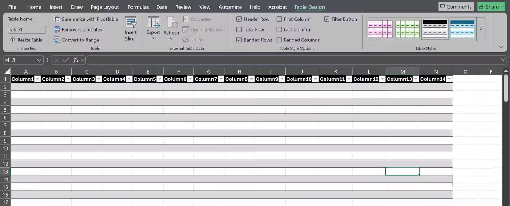
Since most spreadsheet discussions focus on Google Sheets vs. Excel, it makes sense to put pre-built tables in that context. At first glance, there isn't much difference between them. Both Excel and Google Sheets provide you with stylish, functional tables that look clean and are easy to navigate.

 

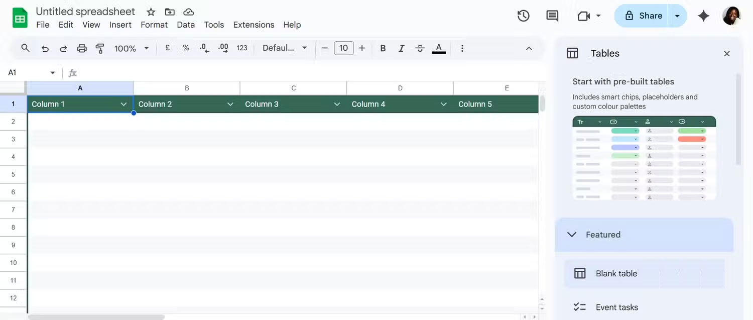
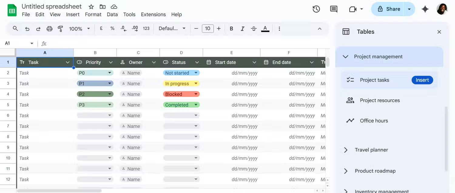
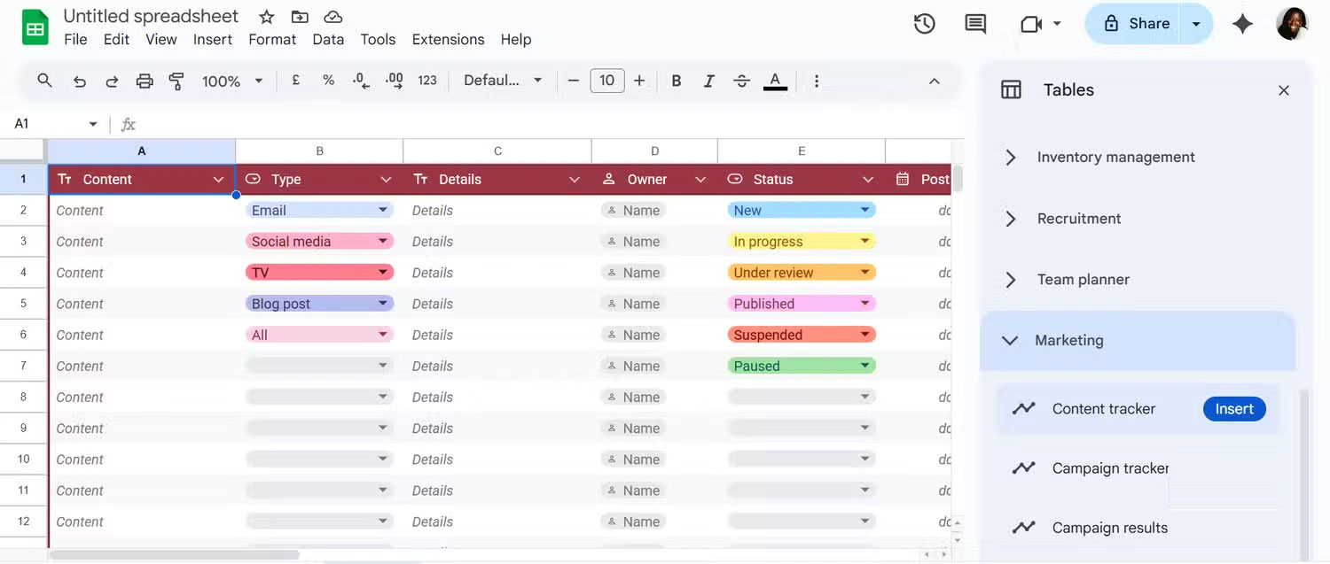
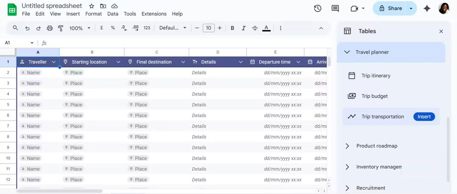
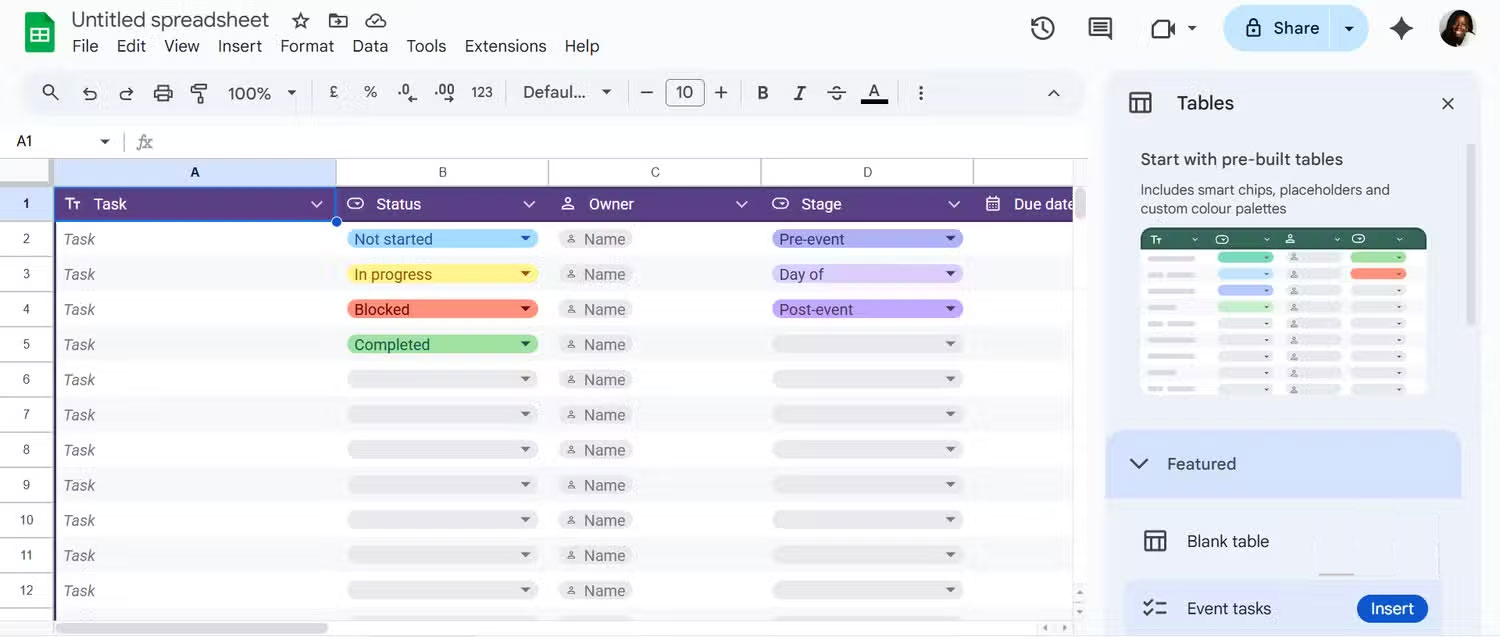
But where Google Sheets really stands out is that you can choose from a library of pre-configured, ready-to-use tables. Are you planning a product launch, tracking customer feedback, or recruiting candidates? There's a template for each, and inserting one is as simple as hovering and clicking. Sheets even lets you preview the template on hover, so you know exactly what you're getting before you drop it into your spreadsheet.

And while the name suggests you're limited to templates, that's not the case. You can also start with a blank table—no placeholders. However, if you use templates, you'll see that some columns are already equipped with smart chips for things like people, files, locations, or even ratings.

Styling is built in, too: Alternate row colors, header and footer formatting, and matching theme colors. Plus, Sheets handles the basics automatically: Your header row and number columns are frozen by default, making your table easier to scan as it grows. If you need to edit, just find the faint freeze line (between the first two columns and below the header row) and drag it to where you want it.

How to set up and work with pre-built tables

Customize table and column settings

 

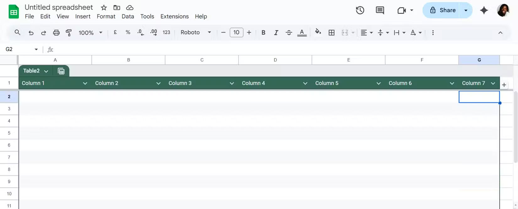
The first thing to do after inserting a table is to expand the rows and columns, which is incredibly easy. To add a row, hover your mouse over the row number until the plus sign appears and click. Or, scroll to the bottom, type a number in the Add more rows at the bottom box , press Enter , and the table will expand immediately. Adding columns is even simpler: Just type in the next empty column, and Sheets will automatically expand the table to fit.

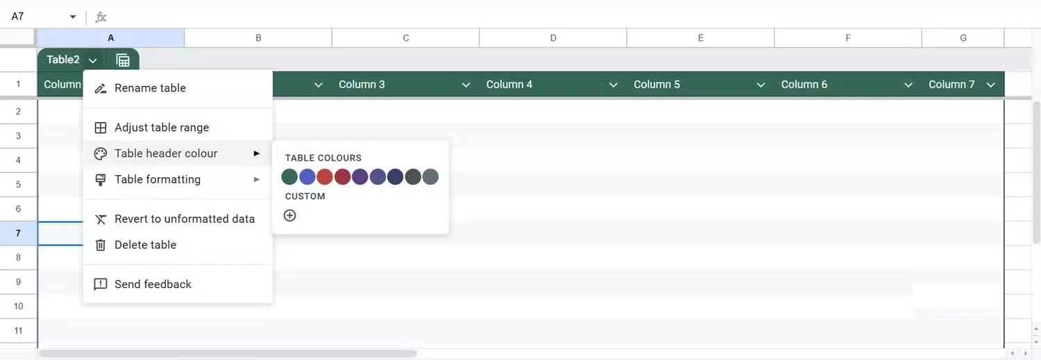
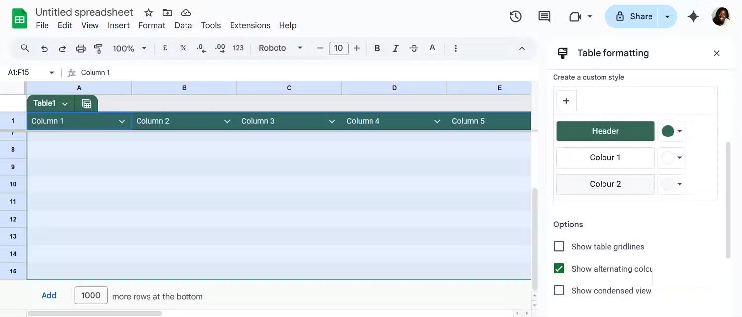
Once you're done, move on to formatting your table and columns. Next to the table name and each column header, you'll see a small down arrow. Clicking that arrow will open the specific table or column menu. From the table menu, you can rename your table, adjust the table range, choose a header color, or format the entire table. You can go straight to Table formatting -> View advanced options to see everything at once.

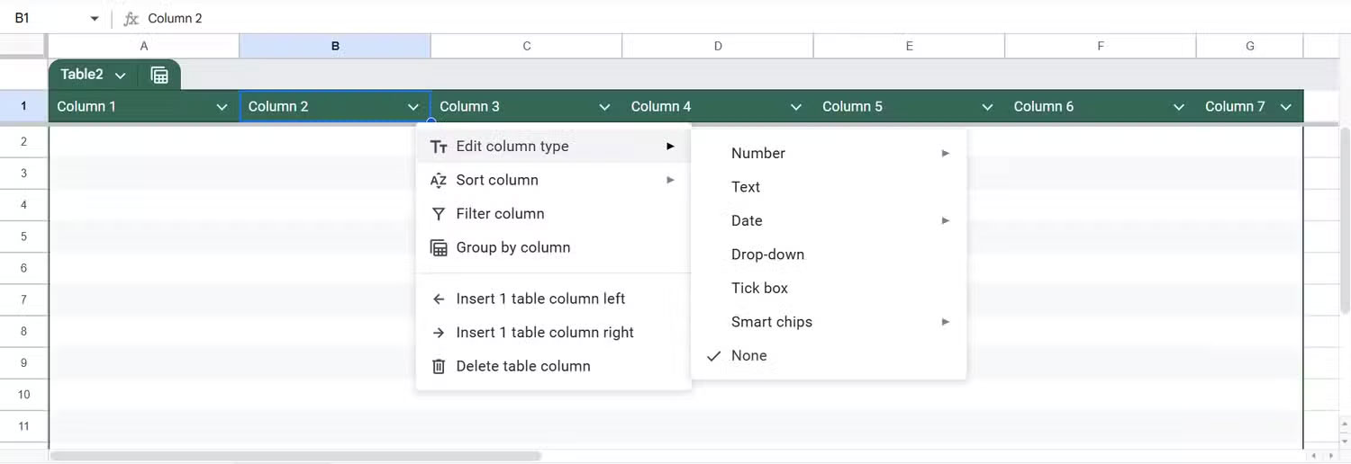
Once your table is set up, tweak your columns. Instead of leaving everything as plain text or numbers, you can define column types like Currency, Dropdown, Checkbox, Smart Chip, etc. Just open the column menu, click Edit column type , and choose the type that fits your data. If someone tries to enter something that doesn't match, Sheets will highlight it with a subtle red highlight. This isn't annoying, but it helps keep your data consistent.

Once you've completed the steps above, it's time to insert data and explore views. Just like Excel's lesser-known Custom Views feature, Sheets lets you save both Group by Views and Filter Views for quick access.

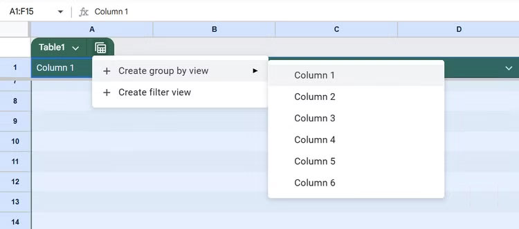
To the right of the table header, you'll see a calculator-like icon that opens the Views menu. From here, you can create a Group by View to organize rows by RSVP status, person, address, or any other column. That way, you can expand or collapse sections for easier review. Once you've grouped, Sheets will prompt you to save the view. If you skip saving, the view will still be active, but only temporarily. The view will be deleted when you reopen the sheet.

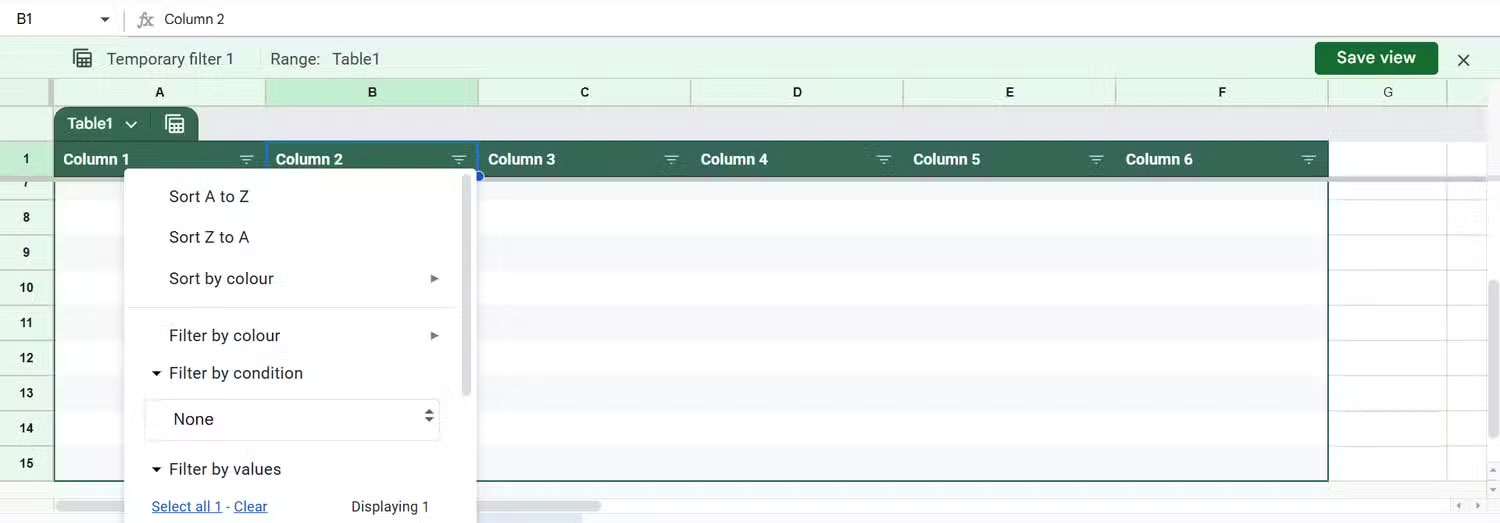
Similarly, you can create a filter view. Click Create filter view and sort or filter the data as you like by launching the column menu. You will find simple sorting and filtering options. Then, click Save view .

With saved filter views, you or anyone with view access can analyze a subset of data without changing what the rest of the team sees.