7 Excel Functions You Should Learn Besides SUM and VLOOKUP

When writing formulas in Excel, SUM and VLOOKUP are basic functions for beginners. However, since Excel has more than 400 functions, it is beneficial to have a better understanding of extremely useful functions, especially when you want to become an intermediate and more advanced user. Let's explore the functions that will help simplify your Excel workflow even more in the following article!

 

The COUNT function provides a better way to count cells.

If they contain numeric data

 

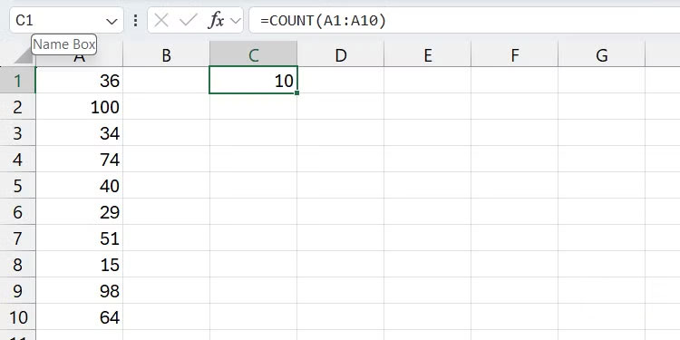
The COUNT function counts all cells with numeric values ​​and returns the result. This saves you the effort of manually counting, which can be tedious and time-consuming in large data sets.

=COUNT(value1, value2, . value_n)

The example formula below will return 10 if all cells contain numbers.

=COUNT(A1:A10)

The AVERAGE function simplifies calculating average values.

Suitable for all ranges

 

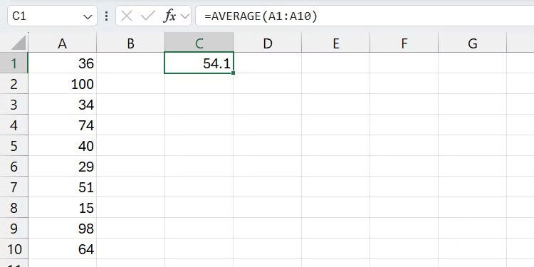
As its name suggests, the AVERAGE function calculates the average (arithmetic mean) by adding all the numeric values ​​in a range and dividing by their total.

=AVERAGE(value1, value2, . value_n)

For example, here is the formula to find the average of the values ​​in cells A1 through A10:

=AVERAGE(A1:A10)

The MIN function finds the smallest value in a range.

There is also the MAX function.

Let's say you have a large data set and need to find the smallest value. The MIN function is the fastest way to do this.

=MIN(value1, value2, . value_n)

Here is an example of how the function works:

=MIN(A1:A10)

 

On the other hand, if you want to find the largest value in a range, use the MAX function.

=MIN(value1, value2, . value_n)

The SUMIF function is a smarter version of the SUM function.

Need some conditional logic

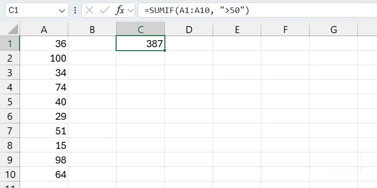
The SUM function simply adds up any numeric values ​​you supply to it. However, the SUMIF function only adds up those values ​​if they meet a specific criteria. This function essentially combines the SUM and IF functions in Excel, so you don't have to manually sort or filter your data before calculating the total.

=SUMIF(range_to_evaluate, criteria, [range_to_sum])

Here, range_to_evaluate is the cells whose values ​​the function should check against the condition specified in the criteria parameter . The optional parameter, range_to_sum , is the specific cells within the range that you want to sum. If you omit this parameter, it will simply sum all the cells within the range that meet the condition.

Here's an example of the function in action. This formula only sums the values ​​in range A1:A10 if they are greater than 50 .

 

=SUMIF(A1:A10, ">50")

There are also variations of the SUMIF function you might consider, including COUNTIF , AVERAGEIF , MINIF , and MAXIF. Some versions allow you to specify multiple criteria, such as SUMIFS, COUNTIFS, and AVERAGEIFS.

The SUBTOTAL function provides a more compact aggregation.

Unnecessary data won't ruin your calculations

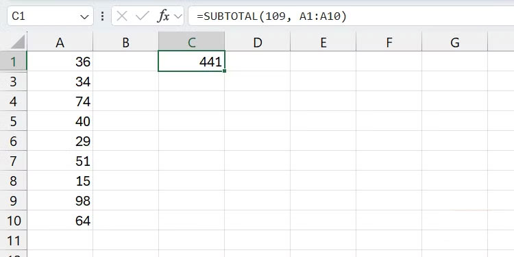
SUBTOTAL is used by Excel pros because it intelligently excludes filtered or hidden data, whereas SUM and similar functions include everything. This makes it an ideal choice when you're working with dynamic data sets, especially when hiding and filtering ensures accuracy.

=SUBTOTAL(function_code, range)

The function_code parameter is a number from 1-11 or 101-111 that specifies the function to use (for example, 1 for AVERAGE, 2 for COUNT, 9 for SUM). Numbers from 1-11 will include all data, while 101-111 will exclude hidden rows. The range parameter is the cells to subtotal.

The example below will sum the range A1:A10 but exclude hidden rows:

=SUBTOTAL(109, A1:A10)

The XLOOKUP function overcomes the disadvantages of VLOOKUP

Modern search

 

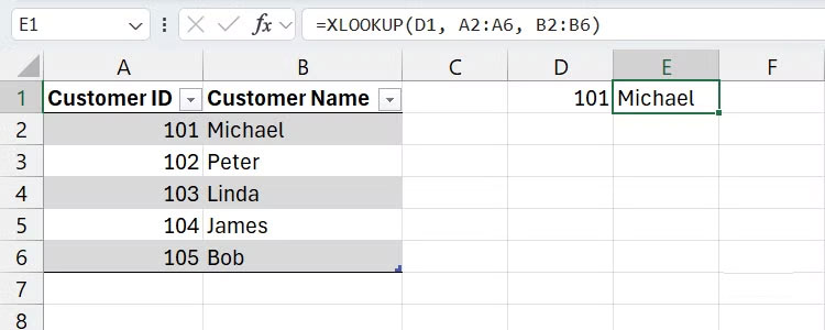
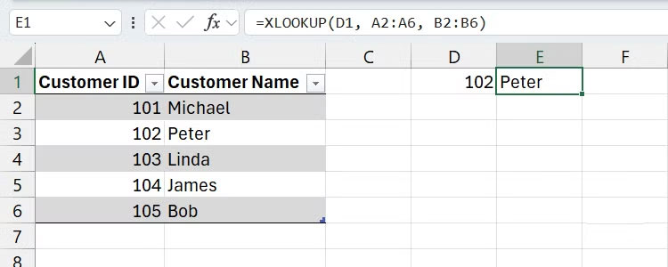
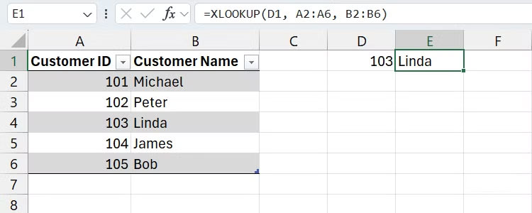
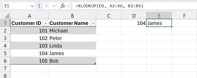
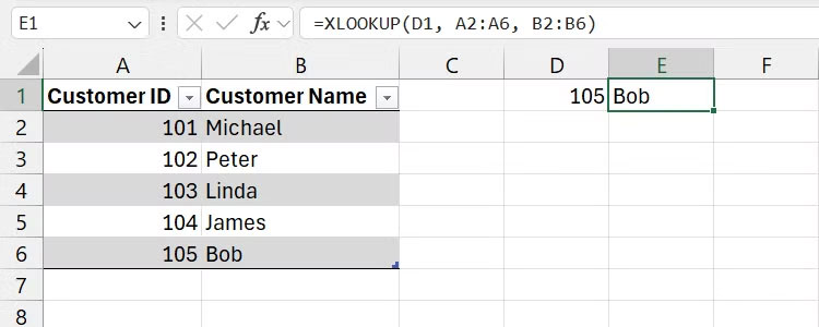
If you're familiar with VLOOKUP, you probably already know its biggest drawback - it can only search from left to right and requires the lookup column to be to the left of the return column. XLOOKUP is more powerful and flexible, allowing you to search in any direction. You don't even need to sort the columns.

=XLOOKUP(lookup_value, lookup_range, return_range)

Where lookup_value is the value you're looking for, lookup_range is where to look for the value, and return_range is the value to return when the value is found. Also, keep in mind that this is the simplified version of XLOOKUP, with the full version including error handling as an optional argument.

Here is an example where range A2:A5 contains customer IDs and range B2:B5 contains customer names. Use XLOOKUP to find the customer name whose ID is found in cell D1 .

=XLOOKUP(D1, A2:A5, B2:B5)

INDEX/MATCH is a classic lookup combination.

Before XLOOKUP

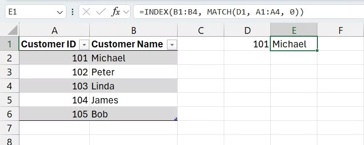
XLOOKUP is not available in versions of Excel older than 2021 and other office suites like LibreOffice or OnlyOffice . So if you want to use XLOOKUP flexibly in these cases, you will need to combine the INDEX and MATCH functions . Moreover, this combination gives you more control over each step of the lookup, although it does not have the error handling capabilities of XLOOKUP.

=INDEX(return_range, MATCH(lookup_value, lookup_range, match_type))

Where, return_range is the range of cells containing the value you want to retrieve, lookup_value is the value you want to look up, and lookup_range is the range of cells in which you want to search for the lookup value. The match_type parameter accepts the following values: 0 for an exact match, 1 for a less than match, and -1 for a greater than match.

Continuing with the XLOOKUP example from the previous section, the INDEX MATCH version would be:

=INDEX(B2:B5, MATCH(D1, A2:A5, 0))

As mentioned earlier, you have control here. For example, you can use the XMATCH function instead of the MATCH function for more advanced lookups. Some people even use the FILTER function if they don't want to manually filter and sort during the lookup.