Basic Excel functions that anyone must know

Using Excel applications, working with basic functions in Excel is very frequent. They help make data calculations directly on the spreadsheet faster and more conveniently. Excel functions are predefined formulas and are already available in Excel, you just need to use them, they are more convenient than many expressions.

The basic functions in Excel that we summarize below such as Excel calculations, statistics, . will be very helpful for you who often have to work on Excel spreadsheets, especially in the field of accounting. , administrative personnel. So make sure you fall into these basic Excel functions. Please refer to me.

1. COUNTING AND CALCULATION

COUNT function

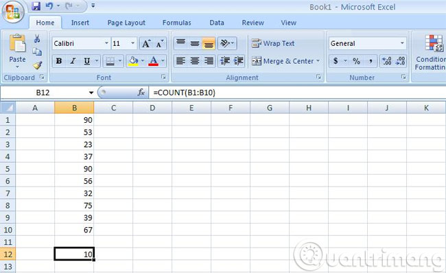
You have a spreadsheet with a huge database and need to know how many cells in a certain area or in the entire spreadsheet contain only numbers, no letters. Instead of having to sit count manually, you can use the function = COUNT . For example, you need to count from cell B1 to B10, type = COUNT (B10: B10) .

Basic Excel functions that anyone must know Picture 1

Count function COUNTIF with specific conditions

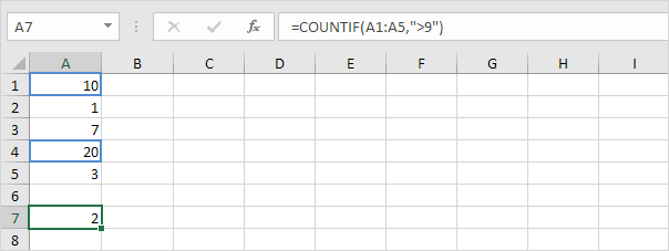
To count cells based on a specific condition (for example, greater than 9), use the following COUNTIF function.

Basic Excel functions that anyone must know Picture 2

Function functions count COUNTIFS with multiple conditions

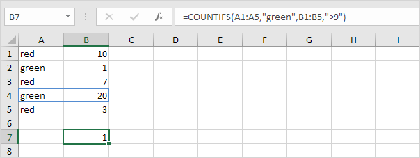
To count cells based on multiple conditions (for example, green and greater than 9), use the following COUNTIFS function.

Basic Excel functions that anyone must know Picture 3

Sum calculation function SUM

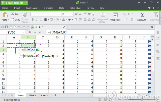
This can be said to be the first function that any new user learning Excel needs to know. Suppose, you want to add the numbers in cell A2 and B2 together, then display the result in cell B3. To do so, simply move to cell B3 and type the phrase " = SUM " and select the = SUM function that appears in the pop-up list.

Basic Excel functions that anyone must know Picture 4

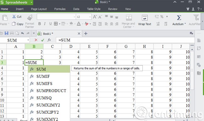
Next, press the Ctrl key along with the mouse click on cells A2 and B2 and then press the Enter key. The result of the sum of the two numbers in two cells A2 and B2 that you just selected will appear immediately in cell B3. You can use the SUM function to calculate the sum of two or more cells, only with the operation to add the necessary cells into the content of the function.

Basic Excel functions that anyone must know Picture 5

The SUMIF function is conditional

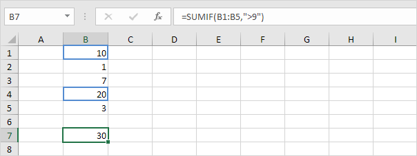
To sum cells based on a condition (for example, greater than 9), use the following SUMIF function (two arguments).

Basic Excel functions that anyone must know Picture 6

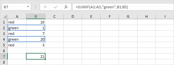
To sum cells based on a criterion (for example, green), use the SUMIF function with 3 arguments (the last argument is the range to be summed).

Basic Excel functions that anyone must know Picture 7

The sum function SUMIFS with many conditions

To sum cells based on multiple conditions (for example, blue and green), use the following SUMIFS function (the first argument is the range of spreadsheets to be summed).

Basic Excel functions that anyone must know Picture 8

The function calculates the average value AVERAGE

The function = AVERAGE does exactly what it calls its name, giving the average value of the selected numbers. For example, if you want to calculate the average value from cell A10 to cell J10, just type = AVERAGE (A10: J10) and press Enter.

Basic Excel functions that anyone must know Picture 9

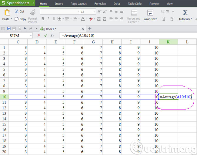
The result in cell K10 is the average value between cells A10 and J10 . Alternatively, you can use the drag and drop cursor and select the data area or you can simultaneously press Ctrl and click on each cell separately in case the cells are not adjacent to each other.

Similar to SUMIF, COUNTIF you can use AVERAGEIF and AVERAGEIFS to calculate the average of cells based on one or more criteria.

Empty cell count function COUNTBLANK

You use this function when you need to count empty cells. Syntax = COUNTBLANK (spreadsheet range to count).

Basic Excel functions that anyone must know Picture 10

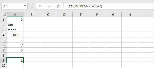
The count function does not empty COUNTA

The COUNTA function has the function to count the number of cells containing any content including digits, letters or symbols, or in other words it is used to count empty cells. Syntax = COUNTA (range of spreadsheet to count).

Basic Excel functions that anyone must know Picture 11

SUMPRODUCT function of total product price calculation

To calculate the total product of the corresponding numbers (the calculation of the total amount of products based on the quantity and the corresponding price of each product) in one or more ranges, use Excel's powerful SUMPRODUCT function.

The following example uses SUMPRODUCT to calculate the total amount spent.

Basic Excel functions that anyone must know Picture 12

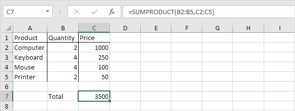
Specifically, SUMPRODUCT has performed the calculation: (2 * 1000) + (4 * 250) + (4 * 100) + (2 * 50) = 3500.

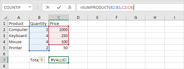
The total scope must be the same size, otherwise Excel will display a #VALUE! Error.

Basic Excel functions that anyone must know Picture 13

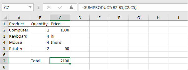
If the value in a non-numeric cell SUMPRODUCT will default to their value of 0.

Basic Excel functions that anyone must know Picture 14

MIN function, MAX

If you want to find a number with the smallest value in a data area, function = MIN can do that. Just type in the phrase = MIN (D3: J13), Excel will return you the smallest number within that range.

Basic Excel functions that anyone must know Picture 15

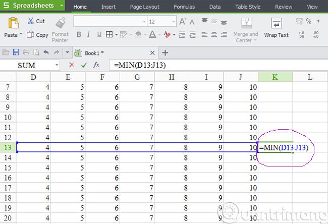
In contrast to the function = MIN just mentioned, the function = MAX will return the largest value in the range to be searched. The syntax of this function is similar to the function = MIN, including the first cell address until the last cell.

2. LOGIC HAIR

IF function

The IF function helps you check if the condition is met, if it is true it will return the correct value, if false returns the wrong value. Formula = IF (condition, "true value", "false value"). To apply to multiple conditions you will have to use the nested IF function.

In the example below, we will check if cell A satisfies the condition greater than 10, if satisfied, returns the Correct value in cell C1, if not satisfied, returns the Incorrect value. In cell C1, enter the function = IF (A1> 10, "Correct", "Incorrect").

Basic Excel functions that anyone must know Picture 16

The IF function returns Correct because the value in cell A1 is greater than 10.

AND function

The AND function will return the correct value if all conditions are satisfied and return the wrong value if there are any false conditions. Formula = IF (AND (condition), "true value", "wrong value)

In the above example, we now combine to check that two conditions, A1 greater than 10 and B1, are greater than 5, if both satisfy, return Correct, otherwise return Incorrect. In cell D1 you enter = IF (AND (A1> 10, B1> 5), "Correct", "Incorrect")

Basic Excel functions that anyone must know Picture 17

The AND function returns the wrong value because cell B1 is less than 5, so the IF function returns the corresponding wrong value here, Incorrect.

OR function

In contrast to AND, the OR returns the correct value if any condition is satisfied and returns the wrong value if all conditions are not met.

Retry the above condition with the OR function. In cell E1 you enter = IF (OR (A1> 10, B1> 5), "Correct", "Incorrect")

Basic Excel functions that anyone must know Picture 18

The OR function returns the correct value because cell A1 is greater than 10, so the result is an IF function that returns the Correct value.

General notes: AND and OR functions can check up to 255 conditions.

Nested IF function

As mentioned above, when you have more than one condition to check, it's time to use the nested IF function. The wrong value will be replaced with another IF function to perform one more test. (If you use Excel 2016, you only need to use IFS.)

Take a look at the examples below:

Enter the formula = IF (A1 = 1, "Bad", IF (A1 = 2, "Good", IF (A1 = 3, "Excellent", "No Valid Score"))) to check the value of cell A1, if equals 1 returns Bad, if equal 2 returns Good, if equals 3 returns Excellent, if another value returns No Valid Score.

Basic Excel functions that anyone must know Picture 19

Basic Excel functions that anyone must know Picture 20

Basic Excel functions that anyone must know Picture 21

Basic Excel functions that anyone must know Picture 22

Enter the formula = IF (A1 <= 10,350, IF (A1 <= 20,700, IF (A1 <= 20,1400,2000))) to check the value of cell A1, if it is less than or equal to 10 then return The value 350, 10

3. DATE MONTH

YEAR, MONTH, DAY function

To enter a date into Excel, use "/" or "-". To fill in the time, use ":" (colon). You can also enter dates and times in the same column.

Basic Excel functions that anyone must know Picture 23

To get the year of the year, you use the YEAR function. Similarly, get the month using the MONTH function and take the date of the DATE function. Formula = YEAR (column contains the year to retrieve).

Basic Excel functions that anyone must know Picture 24

DATE function

To add the number of days in the day, simply use the formula to simply get the box containing the date + with the number of days you want to add, as the example below:

Basic Excel functions that anyone must know Picture 25

To add the year, month, and day to a certain date, you will have to use the DATE function. Formula = DATE (YEAR (cell containing the original date) + number of years to add, MONTH (original date box) + number of extra months, DAY (cell containing original date) + number of days to add).

Basic Excel functions that anyone must know Picture 26

Note: DATE function has only 3 arguments: year, month and day. Excel knows that 6 + 2 = 8 = August, August has only 31 days, so it automatically goes to the next month (August 23 + 9 days to September 1).

The NOW function displays the system time

If you want to enter the current time into a certain cell in the Excel worksheet, use the function = NOW. First of all, move the mouse pointer to any cell and just type the syntax = NOW (). The advantage of this function is that it does not require any parameters inside brackets. The main result is the current time on the computer system.

Basic Excel functions that anyone must know Picture 27

HOUR, MINUTE, SECOND functions

To return hours, minutes, seconds in time, you will use HOUR, MINUTE, SECOND respectively. Formula = HOUR (cell contains the number of hours to take).

Basic Excel functions that anyone must know Picture 28

TIME function

TIME function is used to add the number of hours, minutes, and seconds to the original time, just like the DATE function above. Formula = TIME (HOUR (initial time cell) + number of extra hours, MINUTE (initial time cell) + number of minutes to add, SECOND (initial time cell) + number of seconds to add).

Basic Excel functions that anyone must know Picture 29

Function calculates the number of days between 2 milestones DAYS

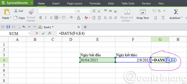
This is a useful formula for calculating the number of days between two milestones, so you don't need to be aware of how many days in each month of the range you want to calculate. For example, cell E4 contains the start date data as of April 30, 2015 and cell F4 containing the end date of September 2, 2015. Please enter = DAYS (F4, E4)

Basic Excel functions that anyone must know Picture 30

DATEIF function

To get the number of days, months, and years of the two timelines in Exel, you will use the DATEIF function. Formula = DATEIF (first timeline, second timeline, "d"). The third argument is what you want to get, "d" is the number of days, you want to get the number of years you replaced by "y", take the number of months instead of "m".

Basic Excel functions that anyone must know Picture 31

Basic Excel functions that anyone must know Picture 32

Basic Excel functions that anyone must know Picture 33

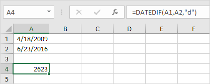
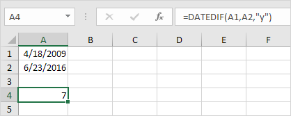
Replace the third argument with "yd" to skip the year, just count the number of days between months of that time period, "md" will skip the month, count only days, "ym" will skip the year, count number of months of difference.

Basic Excel functions that anyone must know Picture 34

Basic Excel functions that anyone must know Picture 35

Basic Excel functions that anyone must know Picture 36

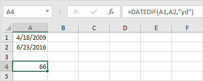
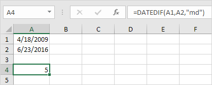
Important note: This function may return false results if the date / month of the 2nd day (located in argument 2) is lower than the date / month of the first day (argument 1). See example below:

Basic Excel functions that anyone must know Picture 37

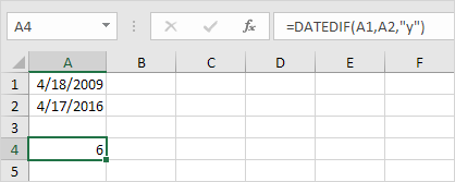
You should then use the formula shown in the image to return the correct result:

Basic Excel functions that anyone must know Picture 38

WEEKDAY function

WEEKDAY function returns the value from 1 (Sunday) to 7 (Saturday), representing the day of the week of the day of the year. For example, 12/18/2017 falls on Monday. Formula = WEEKDAY (cell, date, year).

Basic Excel functions that anyone must know Picture 39

TEXT function

Use the TEXT function to display the day of the week in text. Formula = TEXT (cell containing the date, "dddd").

Basic Excel functions that anyone must know Picture 40

NETWORKDAYS function calculates the number of working days

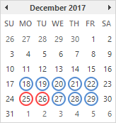
The function = NETWORKDAYS () is used to calculate the number of working days ( ie a 5-day work week ) in a specific time frame. Similar to function = DAYS , use the formula: = NETWORKDAYS (E3, F3).

Basic Excel functions that anyone must know Picture 41

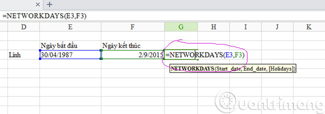
If you provide a holiday list (as in the E1: E2 area of ​​the example below) NETWORKDAYS will return the number of working days (minus weekends and holidays).

Basic Excel functions that anyone must know Picture 42

See the calendar below for a better understanding, red is a holiday, blue is a working day:

Basic Excel functions that anyone must know Picture 43

EOMONTH function

To get the last day of the current date you will use the EOMONTH function. Formula = EOMONTH (cell containing the current date, 0). Using another one instead of taking the last day of the following months, for example, replacing it with 2, then taking the last day of the next 2 months, replacing it with -8 is taking the last day of the previous 8 months. .

Basic Excel functions that anyone must know Picture 44

Basic Excel functions that anyone must know Picture 45

Basic Excel functions that anyone must know Picture 46

4. WORKING METHOD WITH TEXT CHAIN

Append text strings

To join a text string you use the & character, to insert a space, use "" (open quotation marks, close quotation).

Basic Excel functions that anyone must know Picture 47

LEFT function

To get the characters to the left of a string use the LEFT function. Formula = LEFT (cell containing the string to retrieve, number of characters to retrieve)

Basic Excel functions that anyone must know Picture 48

RIGHT function

Use the RIGHT function when you need to get characters from the right side of the string. Formula = RIGHT (cell containing the string to retrieve, number of characters to retrieve)

Basic Excel functions that anyone must know Picture 49

MID function

Use to get the characters starting from (from left to right). Formula = MID (the cell to retrieve, the position to take, the number of characters to retrieve). In this example we get 3 characters, starting with the 5th character.

Basic Excel functions that anyone must know Picture 50

Function LEN

If you want to count the total number of characters, also called the string length in a cell, including letters, numbers and spaces, think of the function = LEN. Formula = LEN (cell containing the string to be counted).

For example, to know how many characters are in cell B4, simply move to any other cell and type in the syntax = LEN (B4) . Immediately, Excel will return a total value of the characters in cell B4.

Basic Excel functions that anyone must know Picture 51

FIND function

Use to find the position of a substring in the string. Formula = FIND ("substring", cell containing string). In this example we find the position of the "am" substring in the "example text" string, and it is in the 3rd position.

Basic Excel functions that anyone must know Picture 52

The SUBSTITUTE function replaces the text

To replace the text in the string with another text you will use the SUBSTITUTE function, with the formula = SUBSTITUTE (cell containing the original string, "original text", "replacement text")

Basic Excel functions that anyone must know Picture 53

The function cuts TRIM gaps

If you have to enter or paste text into Excel such as data from a database, web page, word processing software or other text program, you will notice that the input text has a lot of white space. scattered in the list.

Basic Excel functions that anyone must know Picture 54

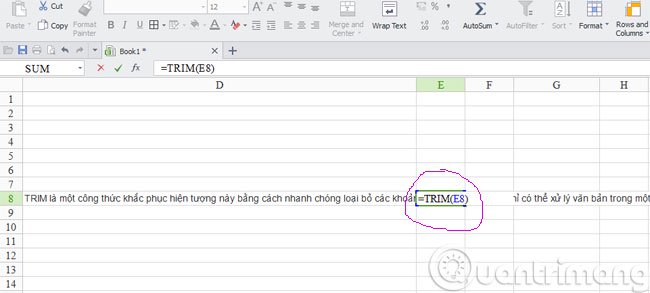
TRIM is a formula to overcome this phenomenon by quickly removing gaps. Function = TRIM can only handle text in a single cell. For example, to perform a space cut in the E8 column, simply type the function = TRIM (E8) once in the F8 box next to it, then copy this formula down until the end of the list.

Function LOWER, UPPER, PROPER to convert uppercase and lowercase letters

You use the LOWER function to convert all capital letters in a string to lowercase, formula = LOWER (cell containing the word to be converted).

Basic Excel functions that anyone must know Picture 55

In contrast, to convert all lowercase letters in a string into uppercase, you use the UPPER function. Formula: = UPPER (cell containing the string to be converted).

Basic Excel functions that anyone must know Picture 56

If you want to capitalize the first words you use the PROPER function. Formula = PROPER (cell containing the string to be capitalized with the first letter).

Basic Excel functions that anyone must know Picture 57

EXACT function to compare two columns

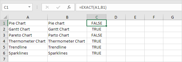
When you need to compare columns to see if their values ​​match, you use EXACT. Formula = EXACT (cell to compare).

Basic Excel functions that anyone must know Picture 58

CONCATENATE function combines content

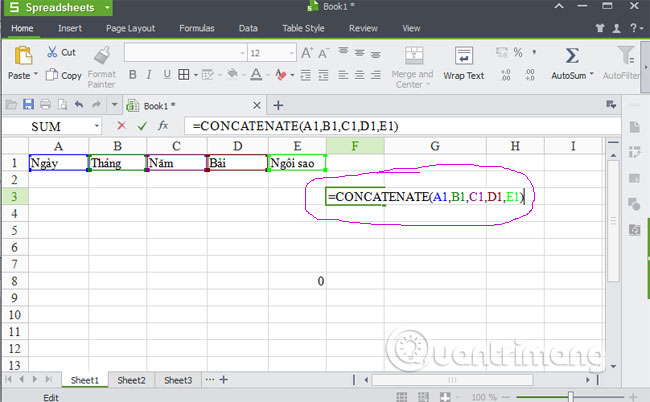
This function will combine the content of two or more cells into a single cell. For example, when you want to enter the date, month, year, card, star into the same cell, type = CONCATENATE (A1, B1, C1, D1) as below

Basic Excel functions that anyone must know Picture 59

5. RESEARCH EXAMINATION AND REFERENCE

Function VLOOKUP

VLOOKUP function searches the values ​​in the leftmost column of the table and returns the value in the same row from the other column you specified. Syntax = VLOOKUP (cell containing search value, table space containing search and return values, column containing return value), can add the fourth argument as the example below.

Basic Excel functions that anyone must know Picture 60

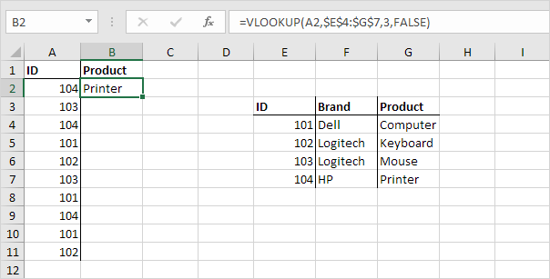
VLOOKUP finds the ID (104) in the leftmost column of the range $ E $ 4: $ G $ 7 and returns the value in the same row from the third column (the third argument is specified as 3). The fourth argument is FALSE to return the correct result or # N / A error if not found.

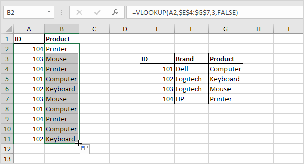
You just need to make one box, then drag VLOOKUP function down to apply to the rows below. Since the reference area remains the same, $ must precede the symbols to create an absolute reference.

Basic Excel functions that anyone must know Picture 61

To better understand how to use VLOOKUP, you can refer to the article: How to use Vlookup function in Excel that TipsMake.com introduced previously.

MATCH function

The MATCH function returns the position of the value in a certain range.

Basic Excel functions that anyone must know Picture 62

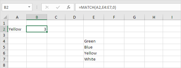
Yellow is found in 3rd place in the range E4: E7. The third argument is optional, you can set this argument to 0 to return the position of the value in the cell or return # N / A if not found.

Function INDEX

The INDEX function below returns a specific value in a two-dimensional range.

Basic Excel functions that anyone must know Picture 63

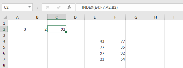
92 is found at the intersection of rows 3 and 2 in the range E4: F7.

The INDEX function below returns a special value in a one-way range.

Basic Excel functions that anyone must know Picture 64

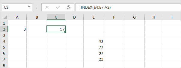
The value 97 is found at the 3rd position of the range E4: E7.

CHOOSE function

CHOOSE function returns the value from the list you specified, based on the required location.

Basic Excel functions that anyone must know Picture 65

In the above example, CHOOSE function returns the value Boat in 3rd place.

1. MS Excel - Lesson 5: Excel formulas and functions
2. How to keep the cells fixed in Excel?
3. How to convert numbers into words in Excel?

You remember to bookmark this post, I will update regularly until the end of "capital" is only ^^