How to Use Hlookup Function on Excel: Excel Hlookup Function

This article examines Excel Hlookup function and explains the main developments, practical implications, and context readers should understand.

Both of these functions are Excel basic functions, with simple usage. However, if you use Vlookup function to search for pre-defined conditions by column, Hlookup function will search by LINE. That is, the user will specify the conditional LINE in Excel and then use the Hlookup function to find the exact value. When using these two search functions, the column or specified LINE element that makes good information will play a role in determining the search direction of the function we want to use. Alternatively, you can combine Vlookup and Hlookup functions with other functions to use.

The following article will guide you how to use Hlookup function on Excel.

• Use VLOOKUP to join two Excel tables together
• How to combine Sumif and Vlookup functions in Excel
• Summary of expensive shortcuts in Microsoft Excel

How to Use Hlookup Excel Function

The syntax of Hlookup function in Excel is

• = Hlookup (probe value, detector value table, order number, search range)

Inside:

• Detector value table: Must be in the absolute address (by selecting the table and pressing F4), when choosing not to scan the title.
• Search scope: If False (0) performs a correct search, True (1) is a relative detection.

We will classify grade point average with the data table below. You will need to use the Hlookup function.

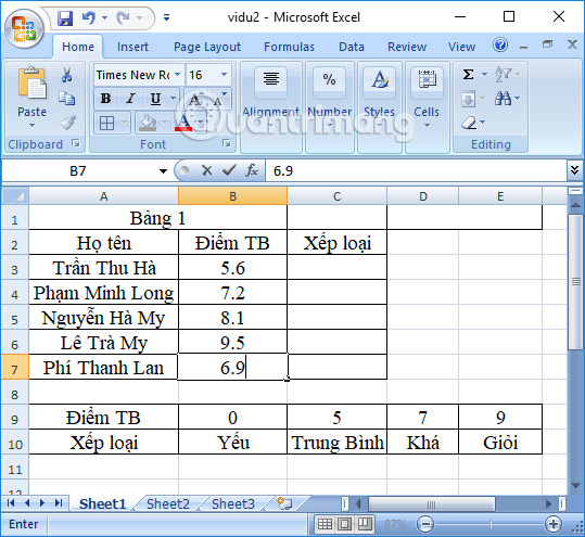
Step 1:

In the first cell of the Sort column of average grades for students, we enter the input formula in cell C3 as: = HLOOKUP (B3, $ A $ 9: $ E $ 10,2,1), then press Enter. The number 2 here will be the Sort LINE in the Excel table with the given condition, 1 will be TRUE relative detection.

Step 2:

The result then we will be graded for the first student as shown below. The formula has been based on students' average scale and grading criteria for students.

We pull down the remaining boxes to complete the average score for students.

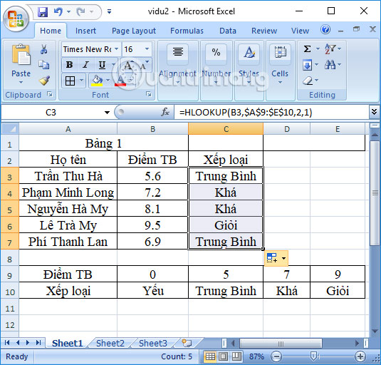
Thus, we have instructed you how to use Hlookup function to search data in the table with given conditions and information. The function will return to the user the exact result based on the conditions set. We can also combine Hlookup with SumIf function with Excek tables that require more data filtering skills.

I wish you all success!