VLOOKUP function to use and specific examples

VLOOKUP is one of the most useful Excel functions but few understand it. In this article, we will help you understand VLOOKUP with practical examples, such as grading students and staff using the VLOOKUP function.

1. These are the most basic functions in Excel that you need to understand

What is the VLOOKUP function?

VLOOKUP function is a function to detect data in Excel. I assume that you already have background knowledge about Excel and can use basic functions like SUM, AVERAGE, and TODAY. One of VLOOKUP's most commonly used functions is a data function, which means it will work on database tables or simply a list of items. The list has many types. You can make a table about your company's personnel, product categories, customer lists, or whatever. And below is a list of products that Company A is selling in the market:

VLOOKUP function to use and specific examples Picture 1

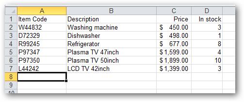
Database tables often have identifiers for each product. In the data table above, the special identification sign is the "Item Code" column. Note: To be able to use VLOOKUP, the data table must have a column that contains an identifier such as code or ID, and must be the first column as shown above.

The formula of VLOOKUP function in Excel 2016, 2013, 2010, 2007, 2003

The VLOOKUP function in Excel has the following formula:

 = VLOOKUP (lookup_value, table_array, col_index_num , [ range_lookup ] ) 

Inside:

1. VLOOKUP: The function name
2. The bold parameters are required.
3. lookup_value: The value used to search
4. table_array: Table contains the value to be searched, to be the absolute value with the $ sign in front, for example: $ A $ 3: $ E $ 40.
5. col_index_num: The order of the column containing the search value on table_array. Example in table $ A $ 3: $ E $ 40, column B contains the value to be searched, col_index_num here will be 2; table $ C $ 3: $ F $ 40, column E contains the lookup value, col_index_num here is 3.
6. range_lookup: As the search scope, TRUE is equivalent to 1 (relative detection), FALSE is equivalent to 0 (absolute detection). This parameter is not required to always be in the formula.

Relative detection is only applicable when the value to be searched in table_array has been sorted in order (ascending or descending or alphabetically). With such tables you can use relative detection, which is similar to using an infinite IF function . For values ​​to be searched that cannot or cannot be sorted, use absolute detection to find the exact value.

Video tutorial using VLOOKUP function

VD1: Use VLOOKUP to evaluate students' and staff's ratings:

Suppose, you have the student transcript as follows:

And the table of ratings is as follows:

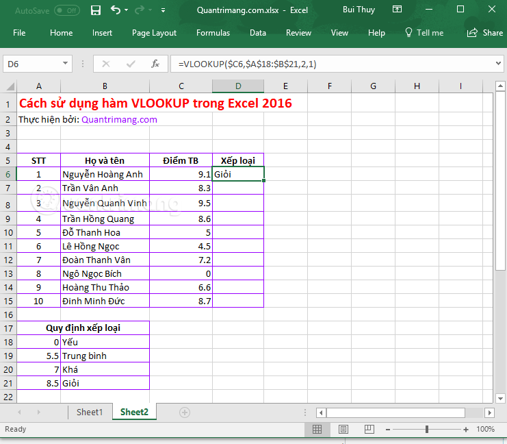
Now we will use the VLOOKUP function to import ratings for students. You notice that the classification table has been sorted from low to high (from weak to good) so in this case we can use relative detection.

In Excel 2 this table is presented as follows:

VLOOKUP function to use and specific examples Picture 2

Here, the value to be searched is in column C, starting from the 6th line. The search range is $ A $ 18: $ B $ 21, the column order contains the search value 2.

In cell D6, enter the formula: = VLOOKUP ($ C6, $ A $ 18: $ B $ 21,2,1). This is a relative detection formula, you can perform absolute detection if you want (or because the rankings are not yet sorted) by adding 0 to the formula like this: = VLOOKUP ($ C6 , $ A $ 18: $ B $ 21,2,0). Press Enter.

VLOOKUP function to use and specific examples Picture 3

Click on cell D6, appear a small square in the lower right corner, click on it and drag down to the end of the table to copy the ranking formula for the remaining students.

VLOOKUP function to use and specific examples Picture 4

At that time, we have the results of using VLOOKUP function to classify students as follows:

VLOOKUP function to use and specific examples Picture 5

Do you have any questions why use $ before C6? $ will help fix column C, only change rows when you drag the formula to the whole table. $ A $ 18: $ B $ 21 to help fix the rating table, making it unchanged when you drag the formula.

Example 2: Use VLOOKUP to detect absolute data

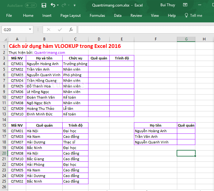
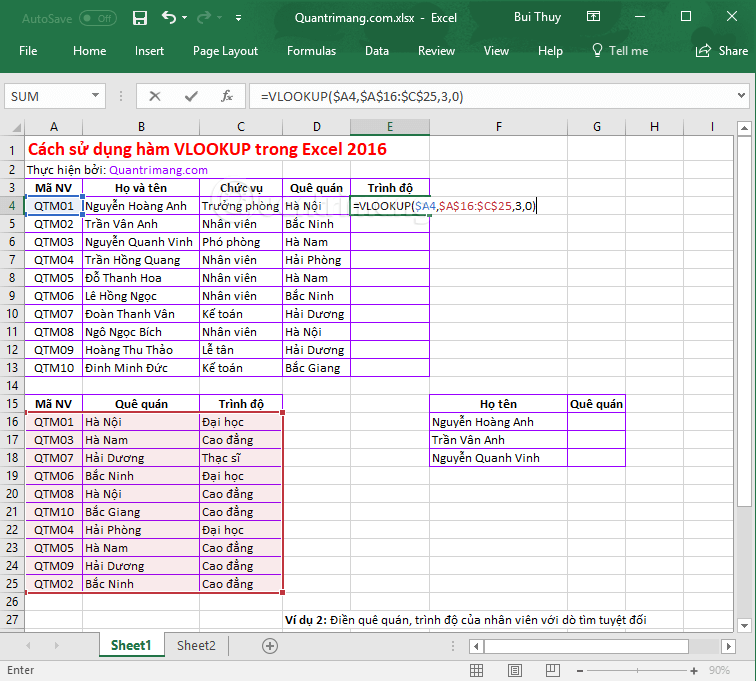
Suppose, you have an employee data table, storing employee code, name and position. Another table stores employee code, hometown, education level. Now you want to fill in your hometown information, what is the level of education for each employee?

Suppose you have the employee table and employee's hometown as follows:

VLOOKUP function to use and specific examples Picture 6

Now you want to fill your hometown information for employees. In cell D4, enter the absolute detection formula as follows: = Vlookup ($ A4, $ A $ 16: $ C $ 25,2,0)

VLOOKUP function to use and specific examples Picture 7

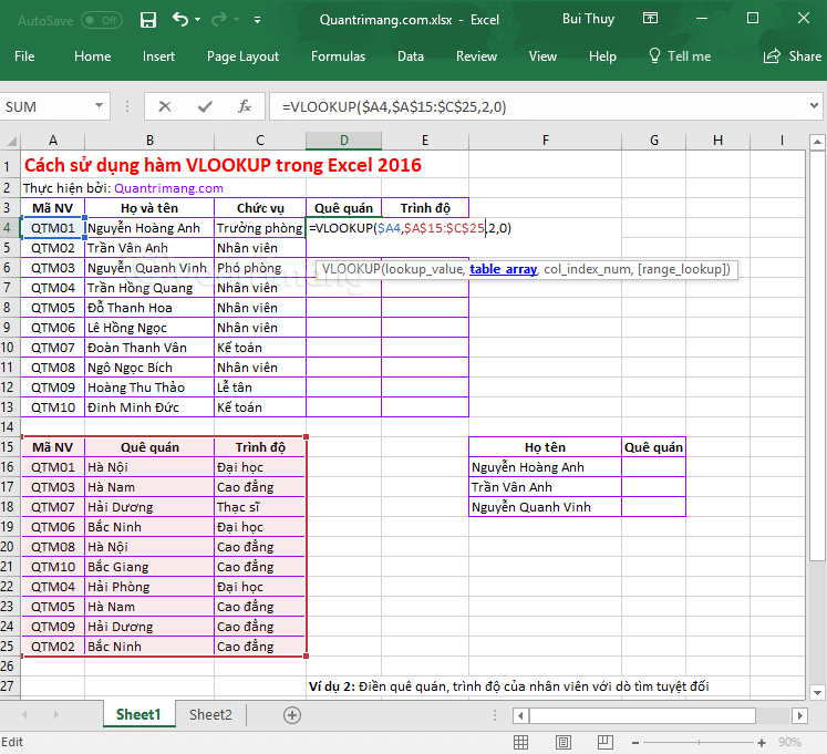
Then press Enter. Click on the small box that appears below the corner of cell D4 and drag down the whole table to copy the recipe for other employees.

VLOOKUP function to use and specific examples Picture 8

To enter qualification information for employees, in cell E4 enter the absolute detection formula: = VLOOKUP ($ A4, $ A $ 16: $ C $ 25.3,0)

VLOOKUP function to use and specific examples Picture 9

You continue to press Enter and drag down to copy the formula for the remaining employees, we will get the following result:

VLOOKUP function to use and specific examples Picture 10

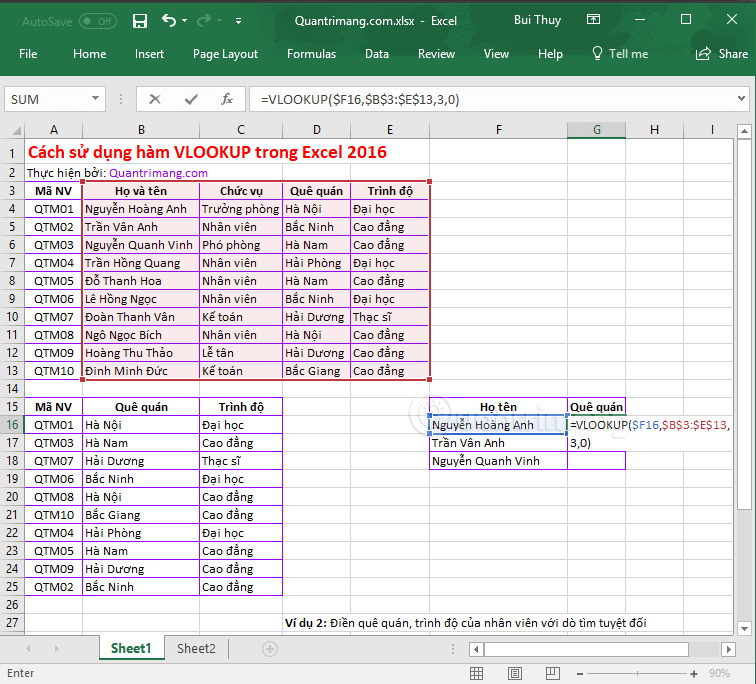
VD3: Use VLOOKUP to extract data

Continuing with the data set of example 2, we will now find the hometown of 3 employees: Nguyen Hoang Anh, Tran Van Anh and Nguyen Quang Vinh. I extracted a new table F15: G18.

This detection will be done on table A3: E13, after it has been filled with native country and level. Now, enter the following absolute detection formula in the box G16: = VLOOKUP ($ F16, $ B $ 3: $ E $ 13,3,0)> press Enter.

VLOOKUP function to use and specific examples Picture 11

Copy the formula for the other 2 employees and get the following results:

VLOOKUP function to use and specific examples Picture 12

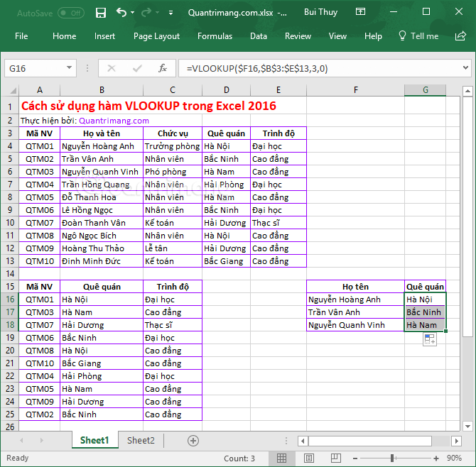
Note in this example, the detection value is in column B, so the detection area is calculated from column B without counting from column A.

VD4: Use VLOOKUP on 2 different Excel sheets

Go back to the data set in example 2 after the employee has completed the qualification and the hometown, we name the sheet as QTM.

VLOOKUP function to use and specific examples Picture 13

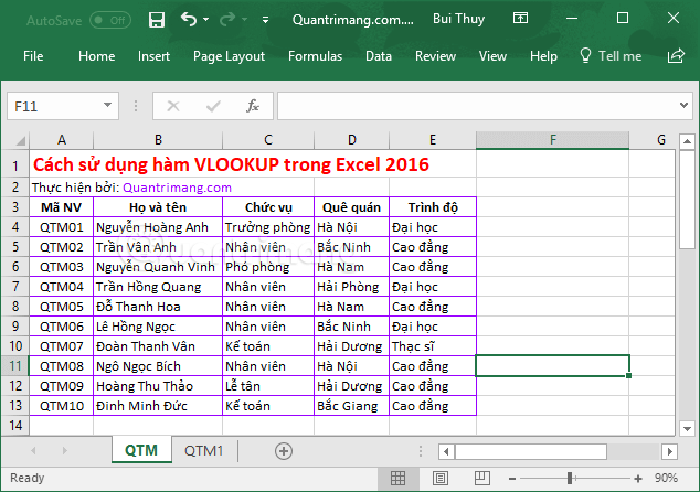
In another sheet of the spreadsheet, naming the TMTM1, you need to get information about your employees' qualifications and positions with the changing order of employees. This is when you see the real power of VLOOKUP.

VLOOKUP function to use and specific examples Picture 14

To search for employee "Level" data, enter the formula: = VLOOKUP ($ B4, QTM! $ B $ 3: $ E $ 13,4,0) in the C4 box of the QTM1 sheet.

VLOOKUP function to use and specific examples Picture 15

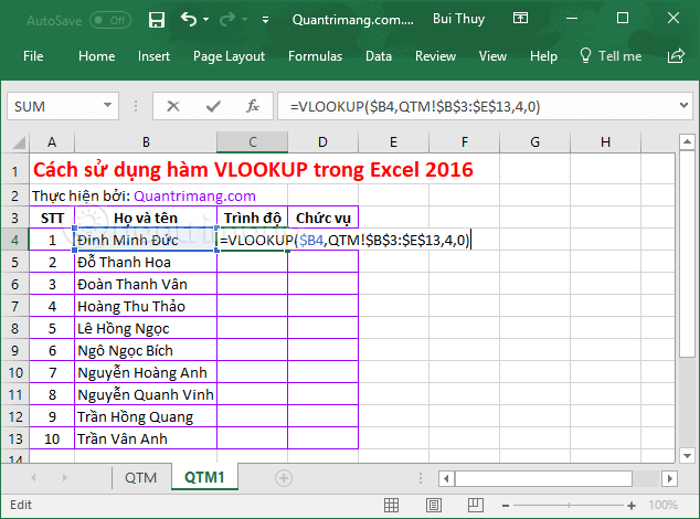
Inside:

1. B4 is the column containing the value used for detection.
2. QTM! is the sheet name that contains the table with the value to be searched, after the sheet name you add the mark!
3. $ B $ 3: $ E $ 13 is a table containing a table search and sheet value (QTM).
4. 4 is the sequence number of the "Level" column, calculated from the "Full name" column on the QTM sheet.
5. 0 is the absolute detection.

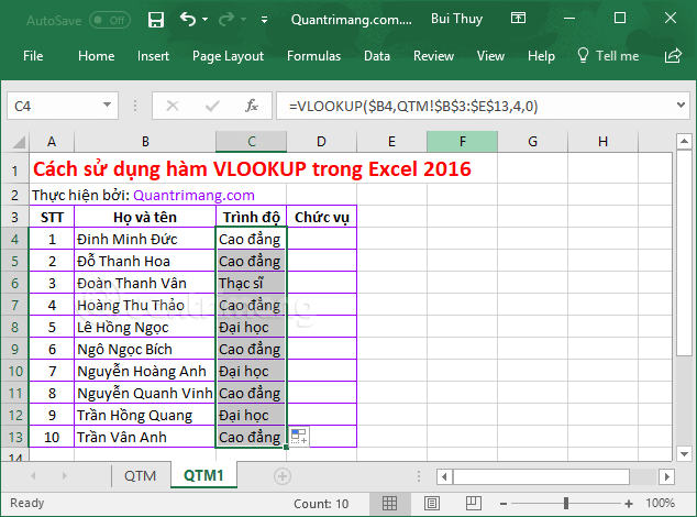
Press Enter, then copy the formula for the rest of the staff in the table, we get the following result:

VLOOKUP function to use and specific examples Picture 16

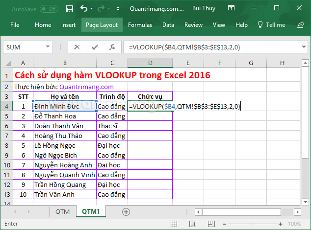
To detect employee "Position" data, in sheet D4 of QTM1, enter the formula: = VLOOKUP ($ B4, QTM! $ B $ 3: $ E $ 13,2,0), press Enter.

VLOOKUP function to use and specific examples Picture 17

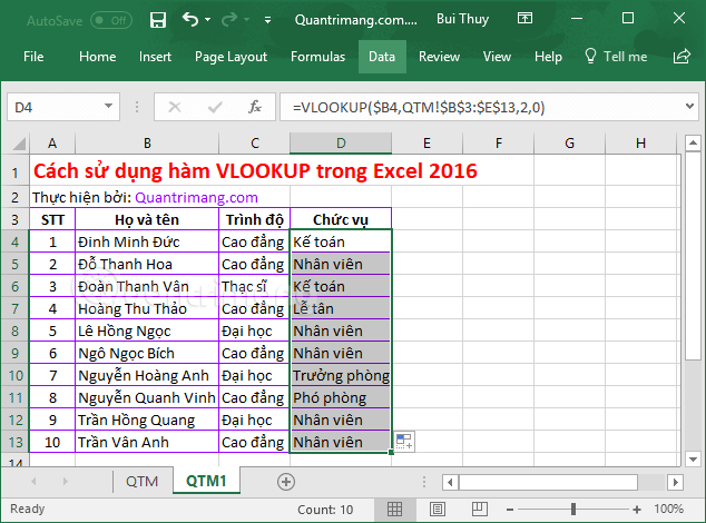
Copy the formula for the remaining employees, we are as follows:

VLOOKUP function to use and specific examples Picture 18

What to do with the VLOOKUP function?

First we need to find the correct answer to the question "what do we use the VLOOKUP function to do?".

VLOOKUP function is used to assist lookup information in a data field or list based on available identifiers.

For example, insert the VLOOKUP function with the product code into another worksheet, it will display the product information corresponding to that code. That information can be description, cost, inventory, depending on the recipe content you write.

The smaller the amount of information you need to find, the harder it will be to write VLOOKUP. Usually you will use this function in a reusable spreadsheet as a template. Each time you enter the appropriate product code, the system will retrieve all necessary information about the corresponding product.

See more:

1. How to use the IF function in Excel
2. How to use AVERAGEIF function in Excel