5 real-world examples demonstrating the effectiveness of the MAP function in Excel.
This article aims to highlight some practical examples demonstrating the power of the MAP function. It can be confusing, as you have to use it in conjunction with LAMBDA functions..
If you're using Microsoft Excel 365, 2021, or 2024, you have access to dynamic array functions. These functions take productivity to a new level thanks to their "spill" functionality. This means a single dynamic array function returns multiple results that spill over into adjacent cells, simplifying complex array operations. One of the functions widely used by Excel professionals is the MAP function .
Specifically, this article aims to highlight some practical examples demonstrating the power of the MAP function. It might be confusing, as you have to use it with LAMBDA functions . However, once you see how it works in practice, you'll realize that the MAP function can save a lot of time. This is especially true if you're dealing with many repetitive tasks.
Multicolumn logic
Handling multiple arrays in a single formula
A common use case for MAP functions is creating multi-column logic. A single formula can handle multiple arrays simultaneously. This means you no longer need to rely on the traditional fill-down method, where you enter the formula into one row and drag down to fill the rest. In doing so, you create thousands of individual formulas that are prone to errors and can impact performance.
The MAP function completely simplifies this. You can import two or more arrays into a single LAMBDA function. This means you can handle complex comparisons in a single formula, ideal for cases like inventory versus reorder point, price versus customer type, or weight versus shipping area.
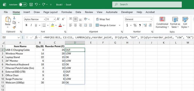
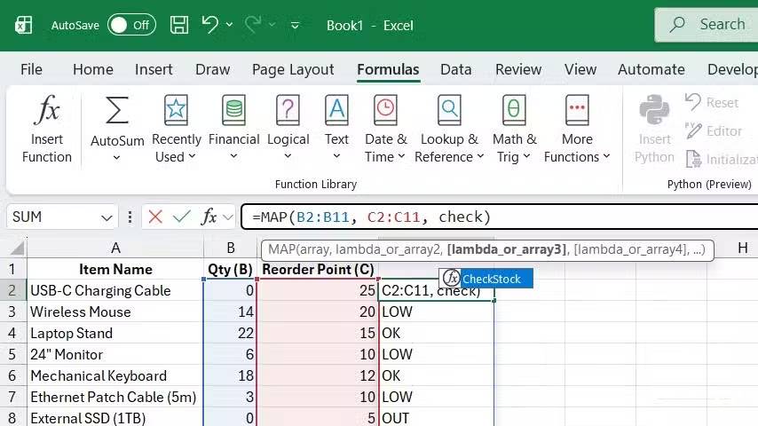
This is the appearance of a formula using the MAP function when comparing inventory with a reorder point. The MAP function evaluates each row of the array and returns the result using a unique, drag-down formula.
=MAP(B2:B11, C2:C11, LAMBDA(qty, reorder_point, IF(qty = 0, "OUT", IF(qty <= reorder_point, "LOW", "OK"))))Minimize errors
Fixing errors is also easier.
Many people have previously managed inventory using Excel, and numerous businesses still do, along with options like Zoho and QuickBooks. The Excel approach often involves filling spreadsheets with numerous IF statements or relying on conditional formatting for visual representation. While these methods are more efficient and easier to use, they also make Excel spreadsheets prone to errors and challenging to maintain.
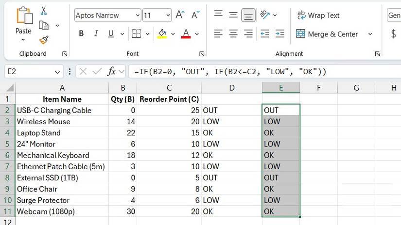
Imagine you've filled in the following formula thousands of lines:
=IF(B2=0, "OUT", IF(B2<=C2, "LOW", "OK"))
If someone accidentally changes one of the parameters in the formula, it can skew your analysis. Finding exactly where the problem lies can be extremely difficult—if not impossible—in large datasets. If you use a MAP function, the results will be copied instead of generating additional formulas.
You can even use the copied cells in other formulas, and everything will work perfectly. However, what you can't do is edit them. Only the cell where you entered the function can be edited, which means no one can accidentally mess up the formula in a random cell and leave you scrambling to fix it. If there's an error, you know where to look.
It helps to make things less prone to errors.
The advantages of named LAMBDA functions
MAP functions take error reduction to a new level with named LAMBDA functions. Specifically, they abstract and mask the logic of complex formulas using descriptive names. This not only means fewer copy-paste errors when reusing formulas, but also fewer unintended changes.
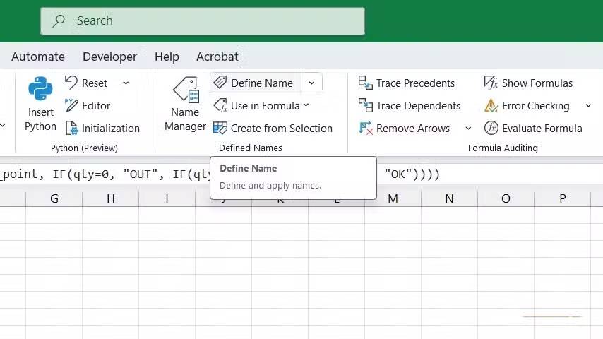
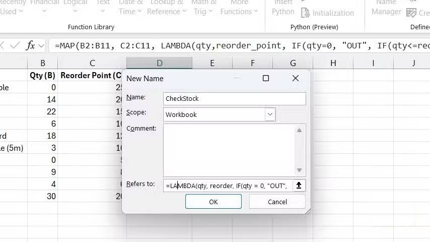
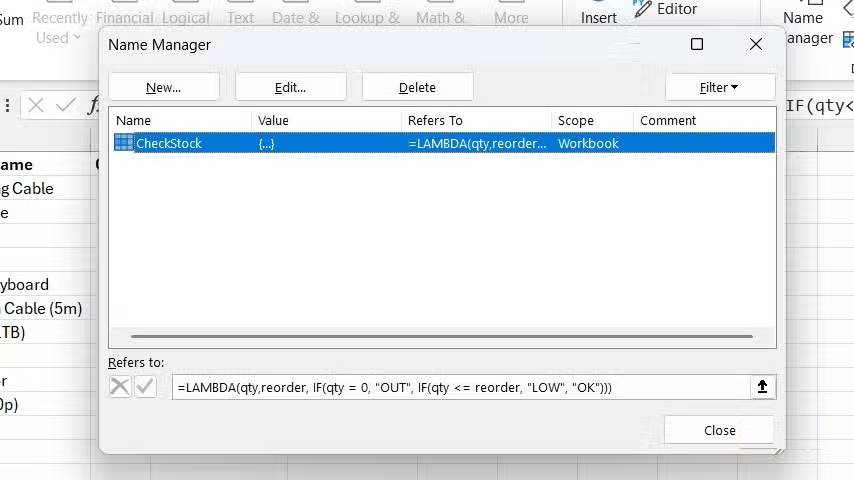
Continuing with the example of inventory versus reorder point, we can create a LAMBDA function named CheckStock using Excel's Name Manager. To do this, select the Formulas tab and click Define Name . Then type CheckStock in the Name field and enter the formula below in the Refers to field .
=LAMBDA(qty, reorder, IF(qty = 0, "OUT", IF(qty <= reorder, "LOW", "OK")))Now, instead of writing that long formula everywhere, the MAP function looks much neater.
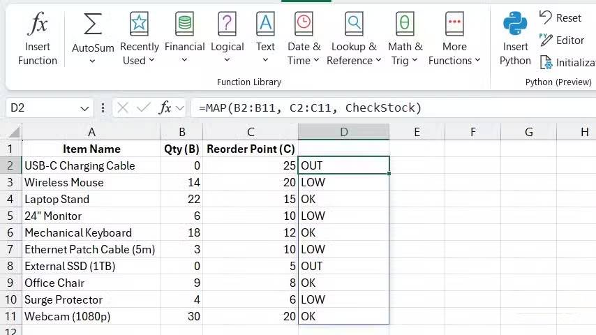
=MAP(B2:B100, C2:C100, CheckStock)Check the calculations in the formula.
The MAP function makes things easier to read.
Another common use case for MAP functions is discounting. A single formula manages all the calculations, eliminating errors across the board. When formulas are scattered throughout a spreadsheet, a single error can be extremely difficult to detect.
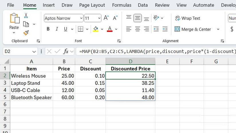
This is an example of using the MAP function to calculate a simple discount. Column B contains the prices, and column C contains the discounts (as percentages):
=MAP(B2:B5, C2:C5, LAMBDA(price, discount, price * (1-discount)))Notice how easy to read the formula is thanks to the LAMBDA function. Without it, the formula for the first discount would look confusing like this, forcing the reader to guess the meaning of the cell references.
=B2 * (1-C2)Even tiered discounts become easier to understand with the MAP function. Yes, you have to sacrifice brevity, but verbosity isn't always bad if the context is right. Anyone who's used Excel for a while can easily understand the formula below:
=MAP(A2:A50, LAMBDA(price, IF(price > 100, price * 0.85, price * 0.95)))Advanced data cleaning
You don't always need to use the fill-down option.
There are many tedious tasks that Excel users hate, and one of the biggest is cleaning raw data. Data cleaning often forces you to rely on auxiliary columns or nested formulas, then fill them down – and many people hate that. As the data grows, you have to remember to expand the formulas, which can lead to errors if you forget.
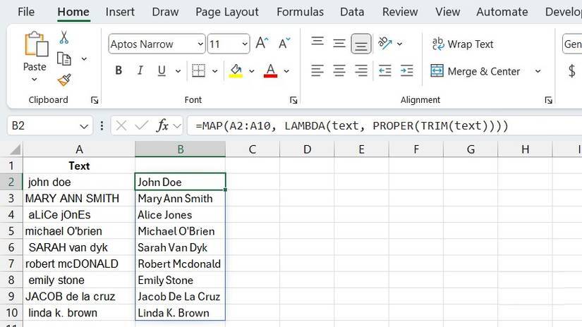
For example, suppose you have a list of products where the names have inconsistent capitalization and leading spaces. This often happens when data comes from multiple different sources. To normalize the text, you can use a formula like the one below and then fill it down.
=PROPER(TRIM(A2))But the problem here stems from manual filling and the risk of formula errors. The MAP function can easily eliminate these issues and keep the spreadsheet looking neat.
=MAP(A2:A1000, LAMBDA(text, PROPER(TRIM(text))))This will automatically spread the fixed text across the entire range - no dragging required.