5 Old Excel Functions You Should Stop Using

Microsoft Excel has a ton of functions, but if you're still relying on VLOOKUP, nested IF statements, or CONCATENATE, you're making your spreadsheets more difficult to manage than they need to be. Microsoft has new, more powerful Excel functions that will make you feel like a spreadsheet wizard and make your formulas easier to read.

 

The good news is you don't have to be an Excel expert - these are designed to replace the clunky, outdated functions you may be familiar with. Whether you're looking up data, building dynamic lists, or working with text, Excel has better built-in tools to save you time.

5. Replace the limited VLOOKUP function

XLOOKUP is much more flexible

 

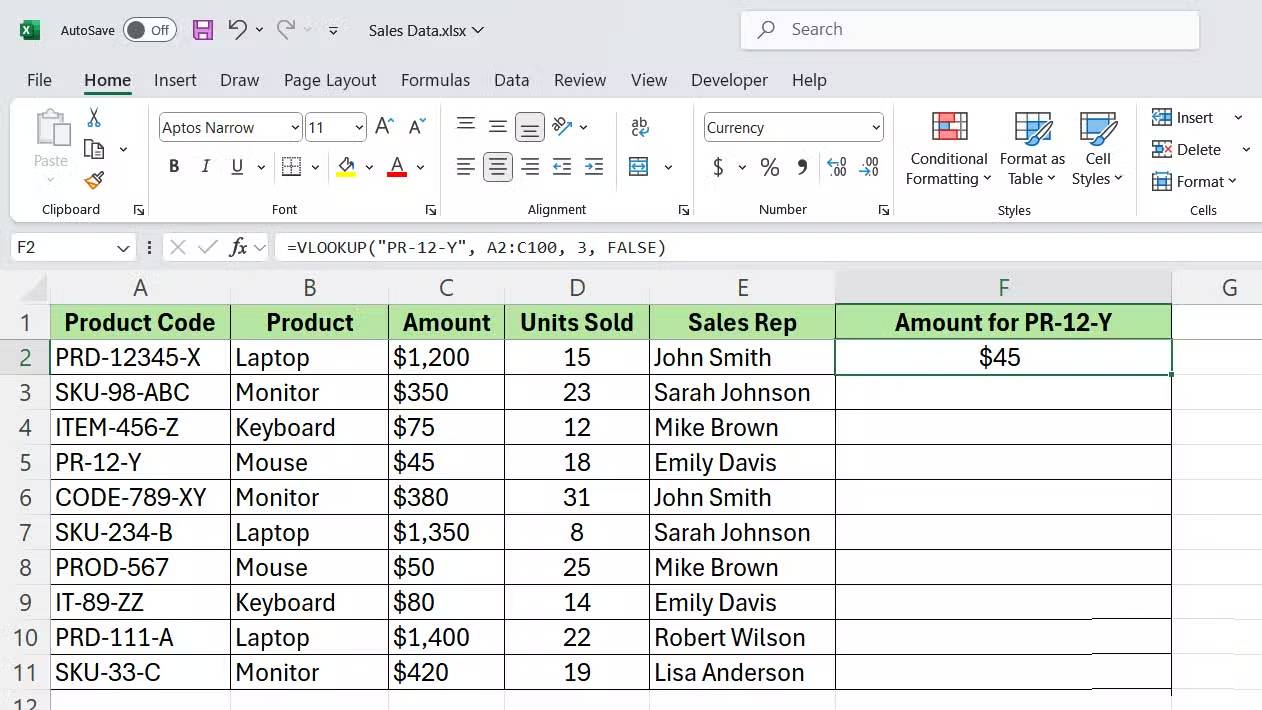
VLOOKUP has been a popular function for looking up data in Excel for years, but it has its limitations. You can only look up in the leftmost column and return a value in the rightmost column. If your lookup column is not on the leftmost, you will have to reorder the entire table or add support columns.

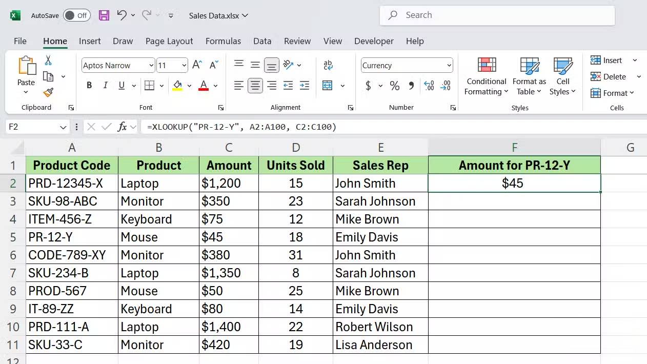
XLOOKUP fixes all of that. It can look up anywhere in a table and return a value from any column—whether it's on the left, right, or somewhere else. Plus, the syntax is simpler and easier to remember.

Compare the syntax as follows:

VLOOKUP:

=VLOOKUP(lookup_value, table_array, col_index_num, [range_lookup])​​

1. lookup_value : The value you are looking for.
2. table_array : The range that contains your data.
3. col_index_num : Number of columns to return (counting from left).
4. range_lookup : TRUE if approximate match, FALSE if exact match.

XLOOKUP:

=XLOOKUP(lookup_value, lookup_array, return_array, [if_not_found], [match_mode], [search_mode])

1. lookup_value : The value you are looking for.
2. lookup_array : The column you want to search.
3. return_array : The column to return the results.

You can also use the following optional parameters:

1. if_not_found : Custom message if no match is found.
2. match_mode : Exact match (0) or other match types.
3. search_mode : Search from top to bottom or back.

4. Eliminate messy nested IF statements

The IFS function is much cleaner

 

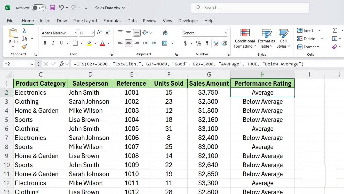
Nested IF statements quickly get out of hand. When testing multiple conditions, you end up with a formula full of parentheses that is nearly impossible to read or debug. Missing a closing parenthesis will break the entire formula.

The IFS function solves this problem by allowing you to test multiple conditions in a single, simple formula. So, no more nesting; just list the conditions and their corresponding results in order.

Compare the syntax as follows:

Nested IF:

=IF(condition1, value1, IF(condition2, value2, IF(condition3, value3, value4)))

IFS:

=IFS(condition1, value1, condition2, value2, condition3, value3, TRUE, default_value)

1. condition1, condition2, condition3 : Logical checks to evaluate.
2. value1, value2, value3 : The result returned if each condition is TRUE.
3. TRUE, default_value : Optional default value when no condition is met.

3. Stop using the tedious CONCATENATE function

Switch to the powerful TEXTJOIN function

CONCATENATE forces you to reference each cell individually and manually enter delimiters, such as commas or spaces, between each cell. If you're combining 5 cells, that's 5 cell references plus 4 delimiters - all entered separately.

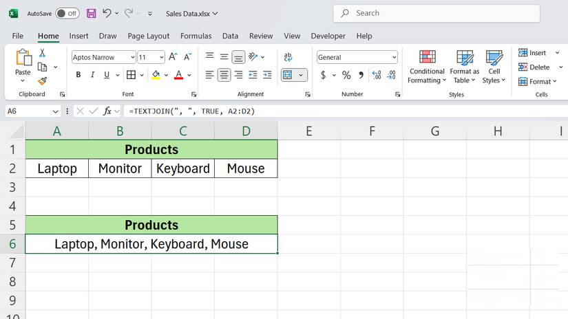
TEXTJOIN handles this in one go. You specify the delimiter once, tell it to ignore blank cells, and then select the entire range. It's much faster to write and easier to edit later.

Here is a syntax comparison:

CONCATENATE:

=CONCATENATE(text1, " ", text2, " ", text3)

TEXTJOIN:

=TEXTJOIN(delimiter, ignore_empty, text1, [text2], .)

1. delimiter : The character or text to insert between each value (comma, space, hyphen, etc.).
2. ignore_empty : TRUE to ignore empty cells, FALSE to include them.
3. text1, [text2], . : The cells or ranges you want to combine.

2. Forget about creating manual lists

 

Using dynamic arrays like FILTER and UNIQUE

Creating a filtered list manually means copying each row or using AutoFilter, then copying and pasting the results somewhere else. If the source data changes, you have to repeat the whole process. This is time-consuming and error-prone.

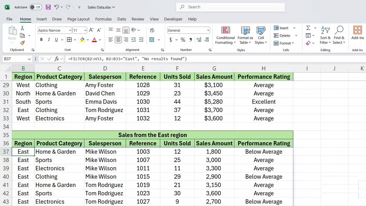
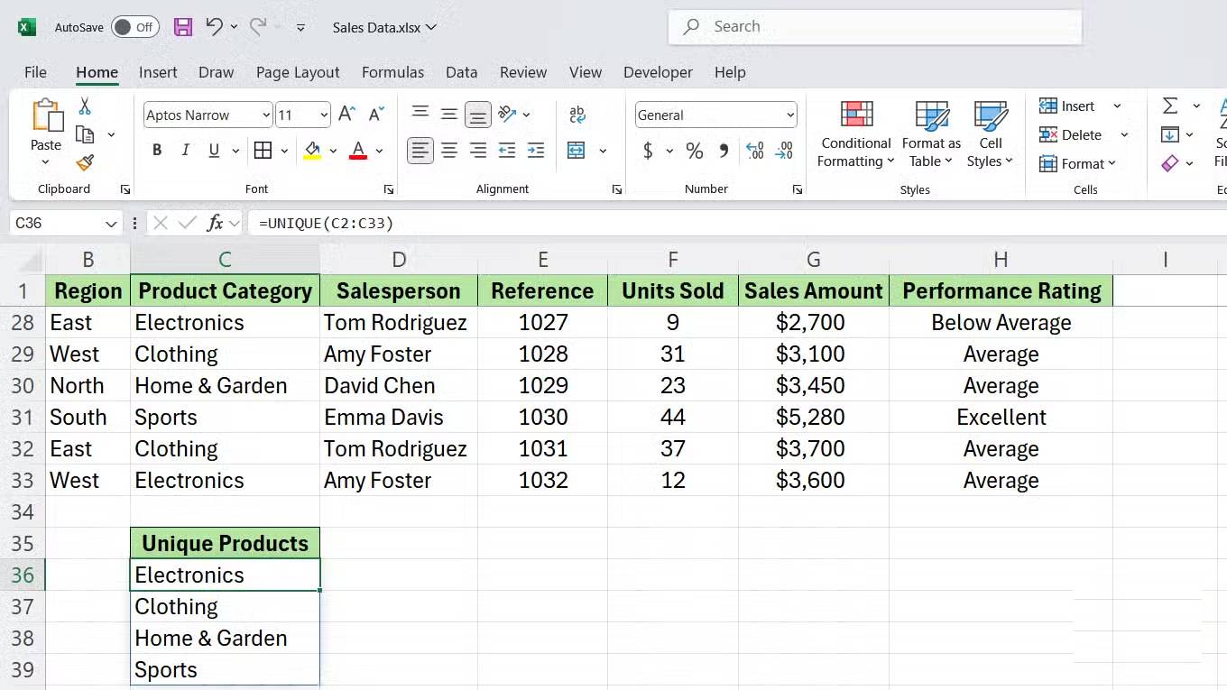
Dynamic array functions like FILTER and UNIQUE automatically create lists that update in real time as your source data changes. You write the formula once, and Excel takes care of the rest. Many people use Excel's FILTER function for everything these days, because there's no need to refresh or manually copy and paste.

Syntax for both functions:

FILTER:

=FILTER(array, include, [if_empty])

1. array : The range of data you want to filter.
2. include : Condition that determines which rows will be included.
3. if_empty : Optional message to display if no results match the condition.

UNIQUE:

=UNIQUE(array, [by_col], [exactly_once])

1. array : The range from which you want to extract unique values.
2. by_col : FALSE to compare rows (default), TRUE to compare columns.
3. exactly_once : FALSE returns all unique values, TRUE returns values ​​that appear only once.

1. Swap LEFT, RIGHT and MID

Because TEXTSPLIT, TEXTBEFORE and TEXTAFTER are more intuitive

 

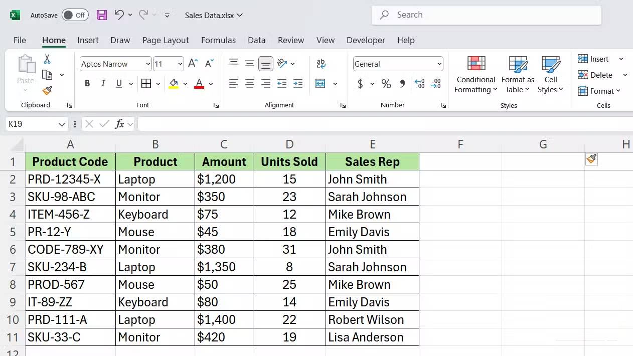
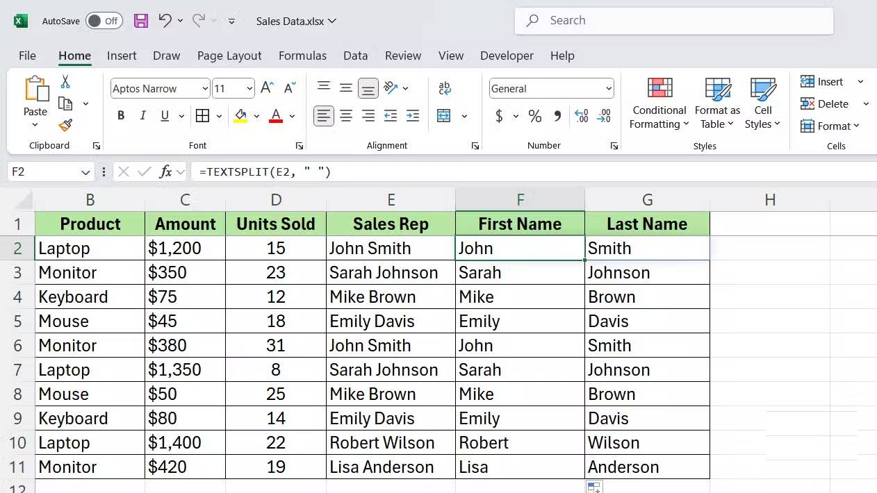
LEFT, RIGHT, and MID require you to count the exact number of characters you want to extract. If your text format changes or its length changes, you will constantly be adjusting the number of characters, and just one miscalculation will break the formula.

The newer text functions—TEXTSPLIT, TEXTBEFORE, and TEXTAFTER—allow you to extract text based on specific delimiters or symbols instead of character positions. They are among the most used Excel functions because of their versatility and ease of understanding at a glance.

Here is the syntax of each function:

TEXTSPLIT:

=TEXTSPLIT(text, col_delimiter, [row_delimiter], [ignore_empty], [match_mode], [pad_with])

1. text : The text string you want to split.
2. col_delimiter : The character that separates columns (comma, space, hyphen, etc.).
3. row_delimiter : Optional character that separates rows.
4. ignore_empty : TRUE to ignore empty values, FALSE to include them.
5. match_mode : 0 for case sensitive, 1 for case insensitive.
6. pad_with : Value to use for empty cells in the result.

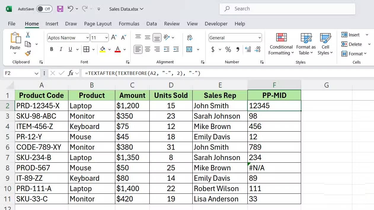
TEXTBEFORE:

=TEXTBEFORE(text, delimiter, [instance_num], [match_mode], [match_end], [if_not_found])

1. text : Text string to search.
2. delimiter : Character or text marking where to stop extracting.
3. instance_num : The number of occurrences of the separator to use (1 for the first, 2 for the second, etc.).
4. match_mode : 0 for case sensitive, 1 for case insensitive.
5. match_end : 0 to search from the beginning, 1 to search from the end.
6. if_not_found : Return value if the delimiter is not found.

TEXTAFTER:

=TEXTAFTER(text, delimiter, [instance_num], [match_mode], [match_end], [if_not_found])

The parameters are the same as TEXTBEFORE, but it extracts the text after the delimiter instead of before it.