Why replace Excel PivotTable with Power Pivot?

PivotTables used to be a failsafe when data was overwhelming, but they always left you squinting at a bunch of numbers. The problem is connecting everything together. Traditional PivotTables forced you to work with separate blocks of data, requiring separate analysis for different aspects of the same data set. Then Power Pivot came along and everything changed.

 

Power Pivot does everything a PivotTable can do.

 

While PivotTables work with single data sources, Power Pivot treats the entire workbook as a connected database. Instead of forcing common Excel functions and formulas to create pseudo connections, you can import multiple related tables and let Power Pivot handle the modeling relationships automatically.

This approach eliminates the endless cycle of updating formulas and fixing broken references that plagued the old workflow. With Power Pivot, adding new data becomes a simple refresh that updates all of your analysis at once.

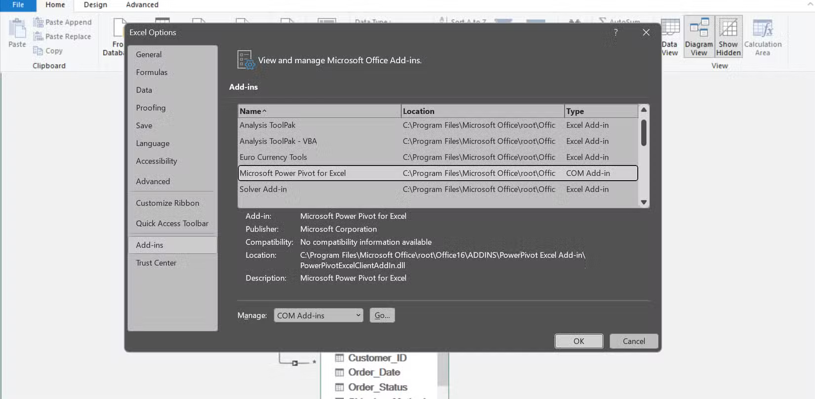
To enable Power Pivot, go to File > Options , click Add-ins , select COM Add-ins from the drop-down menu, and select the Microsoft Power Pivot for Excel check box .

The relational model makes summarizing and analyzing easier than ever.

 

Power Pivot treats data like a real database instead of separate spreadsheets. You simply import each set of data and then define relationships between common fields, allowing Excel to automatically combine the tables and provide consolidated reports without manual lookups. Before using Power Pivot (or any other Excel application), it is important to clean up and prepare your workbook first to ensure reliable results. Many people use Power Query instead of traditional cleanup functions because it scales better and saves me a lot of time cleaning up tables.

To illustrate the power of the relational model, I will use a set of workbooks that I use to populate a backend database during development. This is an e-commerce database with separate spreadsheets for customers, products, orders, and order details, all of which have common fields such as Customer_ID, Order_ID, and Product_ID.

 

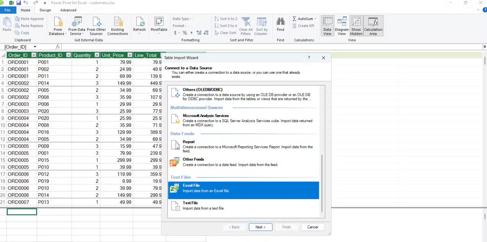
First, open Power Pivot by launching the customer spreadsheet, clicking Power Pivot from the ribbon, and then selecting Add to Data Model under Tables . This will open the Power Pivot menu. From here, add additional spreadsheets by clicking From Other Sources > Excel File , then browse and open the files, click Next , and then Finish . Do this on all of your spreadsheets.

 

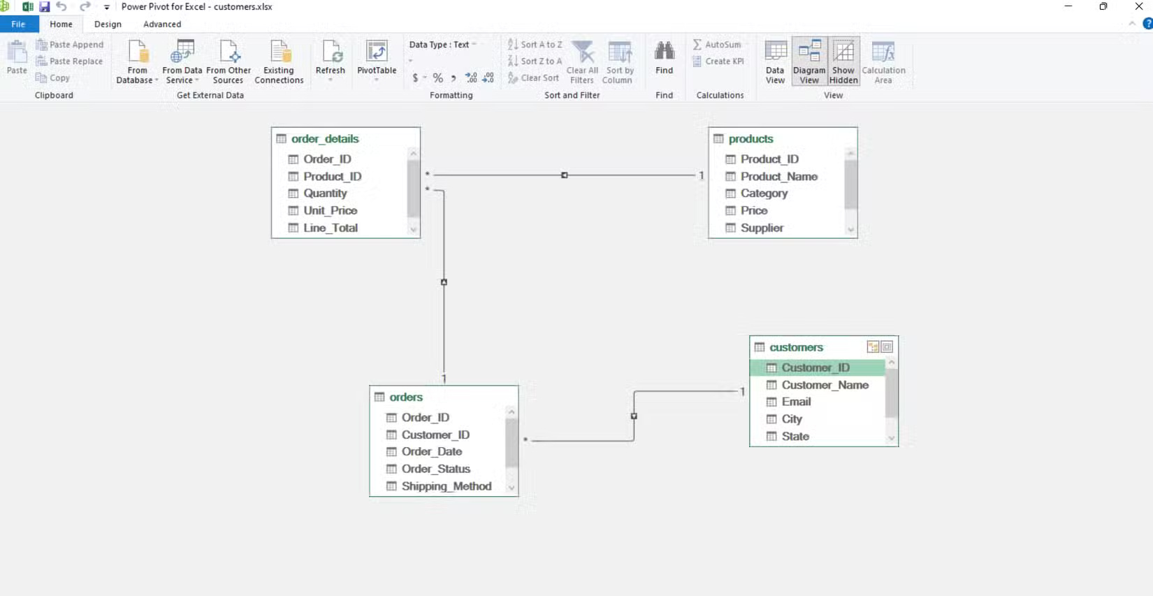
Once you've added all your data, go to Diagram View , located in the Views section of Power Pivot. This displays all four workbooks: customers, order_details, orders , and products. Power Pivot can usually automatically detect and suggest relationships, but you can also define them manually by dragging fields between tables in Diagram View.

In this example, each workbook shares key fields that link the tables together. Both the customers and orders workbooks include a Customer_ID field . The orders and order_details workbooks share an Order_ID field . The order_details and products workbooks use the same Product_ID field . These shared fields form a "one-to-many" relationship. A customer can have many orders, each order can include many products, and each product can appear in many order details. Power Pivot uses these unique identifiers to automatically connect all the data.

DAX calculations allow more flexibility and better insights

 

Now that we have established relationships and demonstrated how easy it is to build reports, it is time to implement DAX. DAX (Data Analysis Expressions) is the formula language behind Power Pivot, specifically designed for advanced data modeling and calculations. Power Pivot's DAX formulas open up analytical possibilities that are nearly impossible with PivotTables.

These formulas allow you to create custom calculations that automate table relationships, performing complex analysis with surprisingly simple syntax. If you're new to DAX, Microsoft's official documentation is a great place to start.

With 3 measures, you can perform calculations that are nearly impossible with traditional PivotTables.

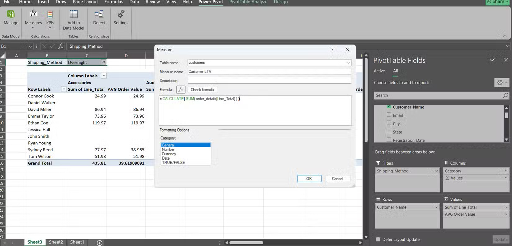
First, let's calculate customer lifetime value. On the Power Pivot toolbar in Excel, click Measures >  New Measure and select the customers table . Name this measure "Customer LTV" and enter the formula:

= SUM(order_details[Line_Total])

Then click OK . Power Pivot will follow the chain from customer to order to order detail and automatically total each customer's purchases.

Next, we want to know the average order size per customer. Again, open New Measure in the customers table , name it "Avg Order Value" and use the formula:

= DIVIDE([Customer LTV], DISTINCTCOUNT( orders[Order_ID]))

Clicking OK will give you a measurement that divides total spend by the number of orders per customer without any supporting columns.

Finally, let's explore shipping options by category. In the products table , create a measure called "Audio Express %" with the following formula:

= DIVIDE( CALCULATE( SUM(order_details[Line_Total]), products[Category] = "Audio", orders[Shipping_Method] = "Express" ), CALCULATE( SUM(order_details[Line_Total]), products[Category] = "Audio" ))

Then, check the box for each measure to see them on the board.

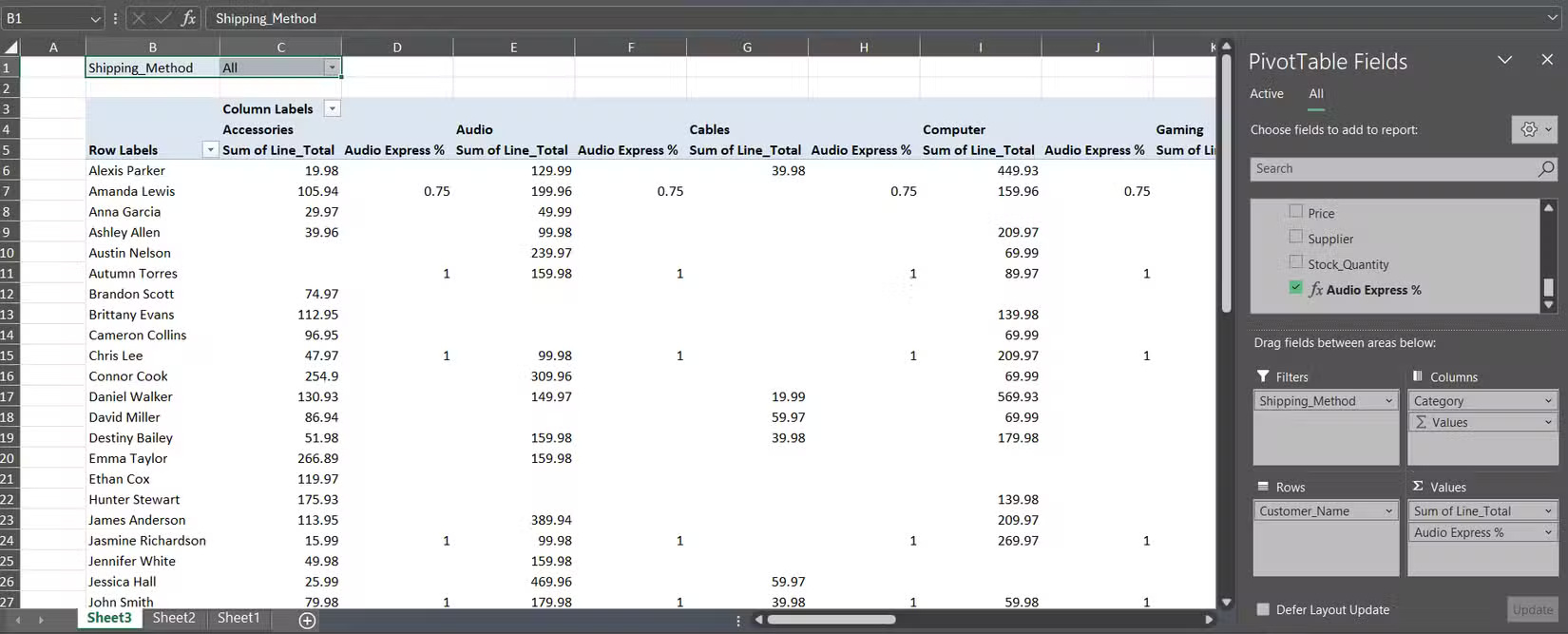
With these DAX measures, you can instantly see total spend by customer by category along with the exact percentage of Audio orders shipped Express in a single PivotTable.