Familiarize yourself with PivotTable reports in Excel

The following article will help you familiarize yourself with PivotTable reports in Excel 2013 accurately and quickly.

To gain a thorough understanding of PivotTable reports, learn the following:

1. What are PivotTable reports?

- PivotTable reports are the most useful feature of Excel that helps you to statistic data according to many different criteria. From there, you save time and effort to produce a detailed report describing the above data.

- A PivotTable reports will turn all data into brief reports that help you determine the information and direction you need for the future.

2. Create a PivotTable reports

2.1 Review the source data.

Familiarize yourself with PivotTable reports in Excel Picture 1

Before creating a PivotTable report, you should review the source data to avoid unnecessary errors.

- The title in the PivotTable report will be taken from the title names of the columns in the data table.

- There should be no blank columns in the source data table to create a PivotTable report.

2.2 Create a PivotTable report dialog box.

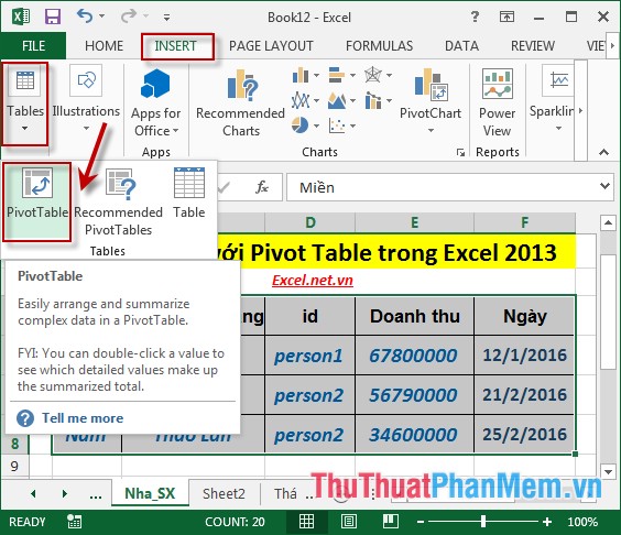
Step 1: Select the data to create a report -> Insert -> Tables -> Pivot Table:

Familiarize yourself with PivotTable reports in Excel Picture 2

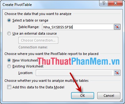
Step 2: After selecting the dialog box appears including the following options:

- Select a table or range: Select the data area to create a report.

- Choose where you want the PivotTable report to be placed: Choose where to save the report:

+ New Worksheet: Save in a new sheet.

+ Existing Worsheet: Save the report in the current sheet.

- After making your selection click OK:

Familiarize yourself with PivotTable reports in Excel Picture 3

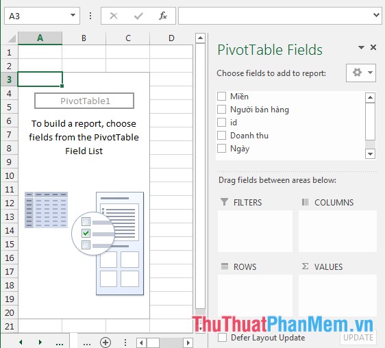
Step 3: After selecting OK the report table appears but there is no data:

Familiarize yourself with PivotTable reports in Excel Picture 4

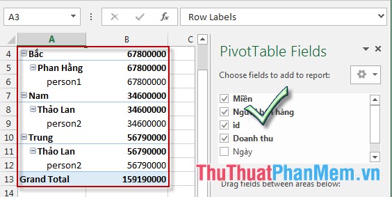
Step 4: Check the name of the fields to create a report -> be PivotTable report:

Familiarize yourself with PivotTable reports in Excel Picture 5

3. Basic PivotTable report.

- PivotTable report includes 2 main parts:

Familiarize yourself with PivotTable reports in Excel Picture 6

+ Layout area for the report: An area that displays all the information of the report.

+ PivotTable Field List : This is where the column headings of source data you want to display on the report and you can optionally select the fields to display on the report.

- In case you want the PivotTable Field List to disappear -> click on the outside of the report, want the report to appear again -> click on the area inside the report layout.

Above is a detailed guide on how to create PivotTable reports in Excel 2013.

Good luck!