Instructions for using PivotTable in Excel - How to use PivotTable

A PivotTable is a tool used to analyze data from different angles and requirements from a list or a table. From the initial huge data block, the PivotTable can help you to aggregate data in groups and collapse data according to your needs.

This is one of the most useful features of Excel. To better understand the PivotTable, refer to the examples below.

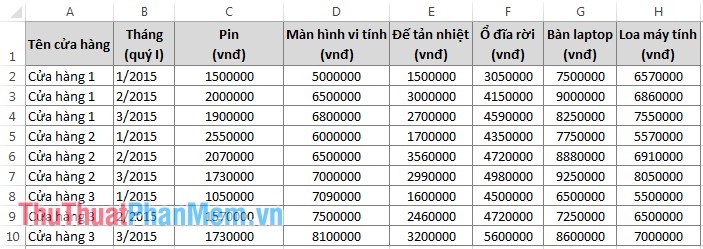
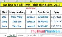
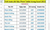
Suppose we have the following data table:

Instructions for using PivotTable in Excel - How to use PivotTable Picture 1

Use PivotTable for simple statistics

Example 1: Using a PivotTable to calculate sales of the Computer Screen items at each Store using the data table above.

Step 1: First, you need to put the cursor in any cell in the data area (or you can select all the data ranges). Then select the Insert tab -> PivotTable .

Instructions for using PivotTable in Excel - How to use PivotTable Picture 2

Step 2: The CreatPivotTable dialog box appears , in the Table / Range section will display the address of the data container. In the Choose where you want the PivotTable report to be replaced section, you choose where you want the PivotTable report to be placed.

New sheet: put in new sheet.

Existing sheet: put in the current sheet, if you select this item, you need to select the address where the PivotTable is located in the Location box .

Then you click OK to create PrivotTable.

Instructions for using PivotTable in Excel - How to use PivotTable Picture 3

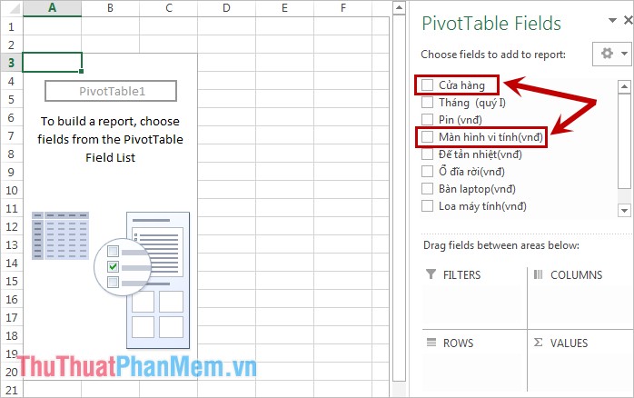
Step 3: At this time, the spreadsheet interface will appear a PivotTable Field List dialog box on the right side of the screen. In this section there are 2 parts: Choose fields to add to report - select the data fields to add to the PivotTable report, Drag fields between areas below - 4 areas to drop the dragged data fields or choose from the choose fields to add to section report ( report filter - data filtering area, column labels - column names, row labels - row names, values - values ​​to display).

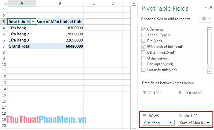
At the request of the example is the sales statistics of the Computer Monitor items at each Store. You have checked 2 boxes of Computer Monitor and Shop .

Instructions for using PivotTable in Excel - How to use PivotTable Picture 4

- If the Computer screen is displayed in the ROWS box , hold down the mouse pointer on that cell and drag it to VALUES .

Instructions for using PivotTable in Excel - How to use PivotTable Picture 5

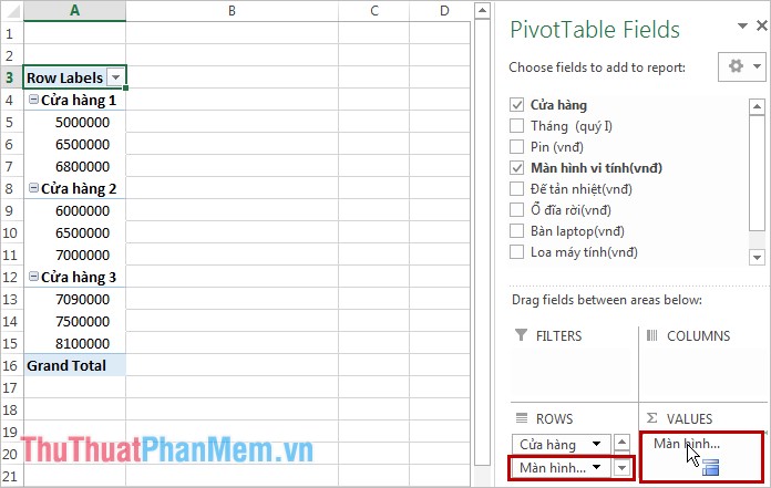
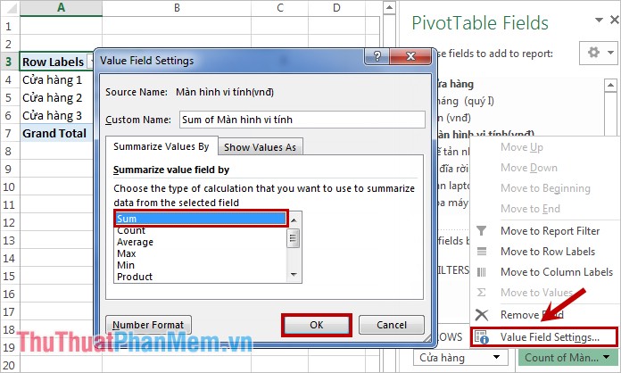
Then click on the cell just dragged to the VALUES section and select Value Field Settings and select the Sum function to statistic according to requirements. For other requirements, you can choose a different calculation function accordingly.

Instructions for using PivotTable in Excel - How to use PivotTable Picture 6

- If the Computer Screen is displayed in the VALUES box as shown below, you have successfully counted.

Instructions for using PivotTable in Excel - How to use PivotTable Picture 7

Note: You can also press and hold on the data at the top to select and drag directly to the 4 regions at the bottom. As the above example, you hold down the mouse in the Store box and drag down the ROWS area, click and hold the mouse on the Computer screen and scroll down to VALUES.

Use PivotTable to statistic data of multiple columns

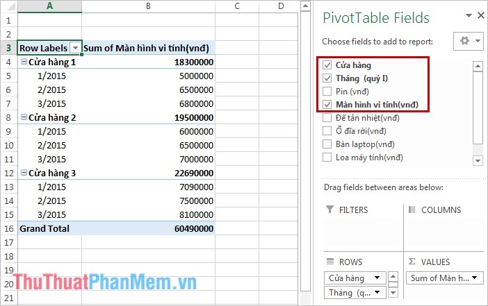
Example 2: Use a PivotTable to display the sales of Computer Screen items over the Months of Stores in the data table above.

First, you also need to create a PivotTable like Step 1, Step 2 in the previous example. Next in the dialog box, PivotTable Field List, select three items: Store, Month, Computer Screen (or you can drag the Store and Month boxes to the ROWS area, Computer Screen into the VALUES area). Your results will be as follows:

Instructions for using PivotTable in Excel - How to use PivotTable Picture 8

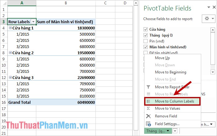
If you want to make comparisons easier, you can move the Month box to the COLUMNS area by left-clicking the Month box in the ROWS area and dragging to the COLUMNS area. Or you can left-click on the Month box in the ROWS area and select Move to Column Labels .

Instructions for using PivotTable in Excel - How to use PivotTable Picture 9

Your results will be as follows:

Instructions for using PivotTable in Excel - How to use PivotTable Picture 10

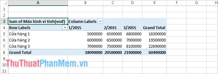
Thus, using PivotTables, you can process and synthesize data quickly from basic requirements or complex requirements. Good luck!