Calculate data in a PivotTable in Excel

The following article details how to calculate data in a PivotTable in Excel.

Creating statistical reports using PivotTable mainly through numbers: summing up quantity, highest sales, lowest . Therefore, the calculation in PivotTable is based on calculating numbers.

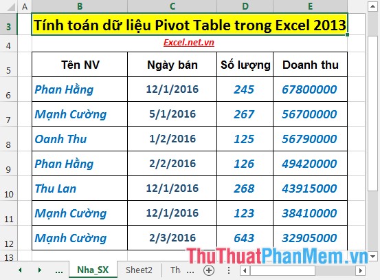
The example has the following data table:

Create a PivotTable report with the above data table reported:

1. Showing data in the report by month.

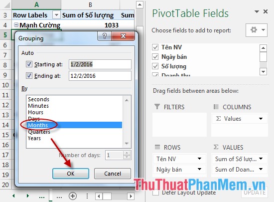
Step 1: Right-click on any day -> Group:

Step 2: The Group dialog box appears, click Months -> OK:

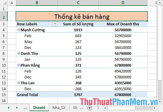
Step 3: After clicking OK -> report is synthesized by month:

2. Convert the calculation to a percentage.

For example, convert the value in the sales column to a percentage.

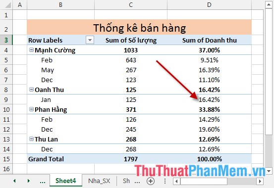
- Right-click on any value in the Sum of revenue column -> Show Values ​​As ->% of Column Total:

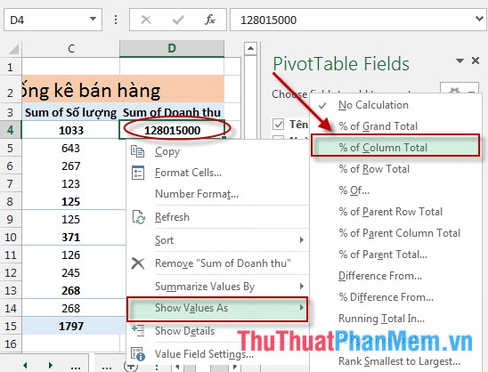
- After selecting the data table, automatically update according to the percentage:

3. Determine the maximum, minimum value, or any calculation in a PivotTable.

For example, find the salesperson with the highest sales.

- Right-click any revenue value in the Sum Of sales column -> Summarize Values ​​By -> Max (or you can optionally choose any calculation such as Average, Min, Product . depending on requirements):

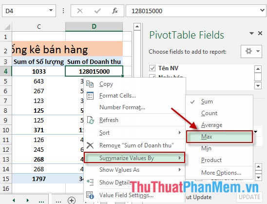
- After choosing the report, automatically update and sort data by revenue and from the report, you can immediately see the highest revenue earner:

Similarly you can do with each other.

Above are detailed instructions and specific examples to help you calculate data in a PivotTable so that you can create multiple reports quickly and accurately for your work.

Good luck!