Sort and filter data
In this lesson, you will learn how to better organize your spreadsheet data and content. You will also learn how to filter data to display only the information you need..
Google Sheets allows you to analyze and work with significant amounts of data. As you add more content to your spreadsheets, organizing the information becomes incredibly important. Google Sheets lets you reorganize your data by sorting and applying filters. You can sort your data alphabetically or numerically, or you can apply filters to narrow down the data and hide certain data from view.
In this lesson, you will learn how to better organize your spreadsheet data and content. You will also learn how to filter data to display only the information you need.
Types of classification
When sorting data, the first important step is to decide whether you want the sorting to apply to the entire worksheet or to a selected area.
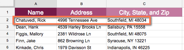
Sorting by worksheet organizes all data in a spreadsheet by column. Related information on each row is stored together when sorting is applied. In the image below, the Name column has been sorted to display customer names alphabetically. The address information of each customer has been stored with their corresponding name.
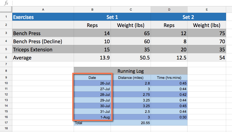
Sorting by range arranges data within a range of cells, which can be useful when working with a spreadsheet containing multiple tables. Sorting one range will not affect other content on the spreadsheet.
How to arrange a spreadsheet
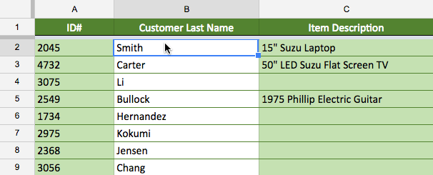
The example will sort a list of customers alphabetically based on their last names. For the sorting to work correctly, your spreadsheet must include a header row, which is used to identify the name of each column. The header row will be fixed so that header labels will not be included in the sorting.
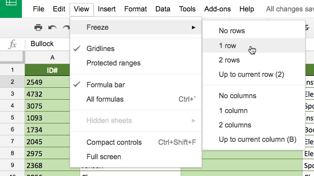
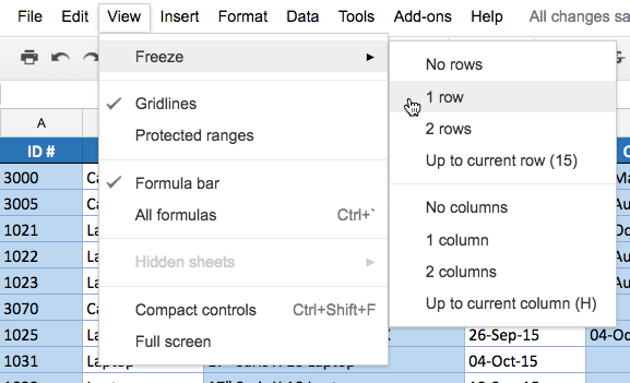
1. Click on View and hover over Freeze. Select a row from the menu that appears.
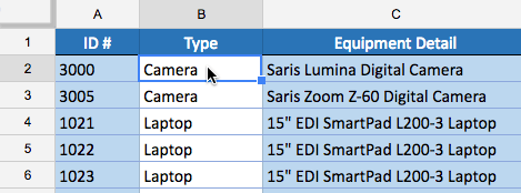
2. The header row is frozen. Decide which column to sort, then click a cell in the column.
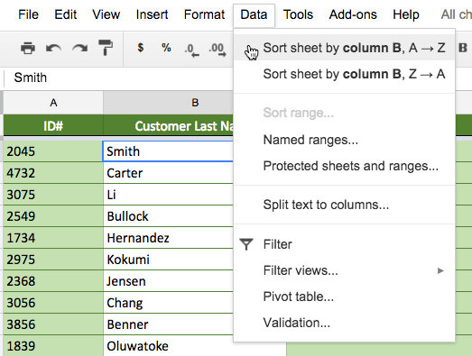
3. Click on Data and select Sort Sheet by column, AZ (ascending) or Sort Sheet by column, ZA (descending) . The example will select Sort Sheet by column, AZ .
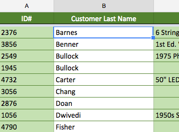
4. The spreadsheet will be sorted according to your selection.
How to sort a range
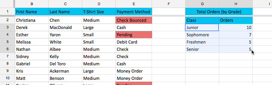
For example, we would select a sub-table in the t-shirt order form to sort the number of t-shirts ordered by class.
1. Select the range of cells you want to sort. For example, we would select the range G3:H6.
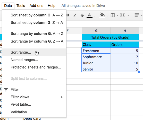
2. Click on Data and select Sort range from the drop-down menu.
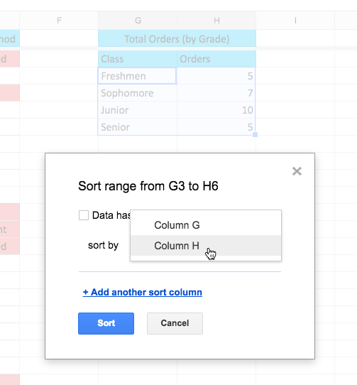
3. The Sorting dialog box appears. Select the column you want to sort.
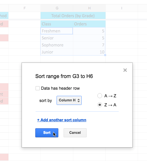
4. Choose ascending or descending order. For example, we will choose descending order (ZA). Then click Sort.
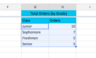
5. The range will be sorted according to your selection (in the example, the data has been sorted in descending order by the Orders column ).
How to create a filter
The example will apply a filter to the equipment log worksheet to only show laptops and projectors available for checkout. For the sorting to work correctly, the worksheet must include a header row, used to identify the name of each column. The header row will be fixed so that header labels will not be included in the filter.
1. Click on View and hover over Freeze. Select a row from the menu that appears.
2. Click on any cell that contains data.
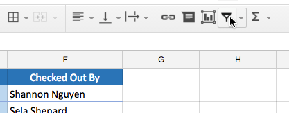
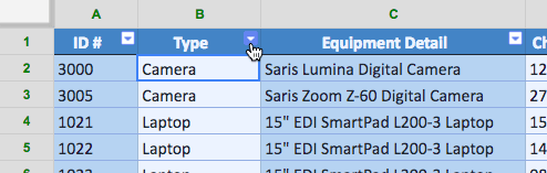
3. Click the Filter button.

4. A drop-down arrow will appear in each column header.
5. Click the drop-down arrow for the column you want to filter. For example, this will filter column B to view only certain types of devices.
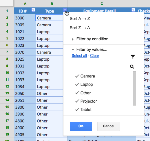
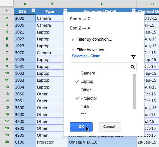
6. Click Clear to remove all checks.
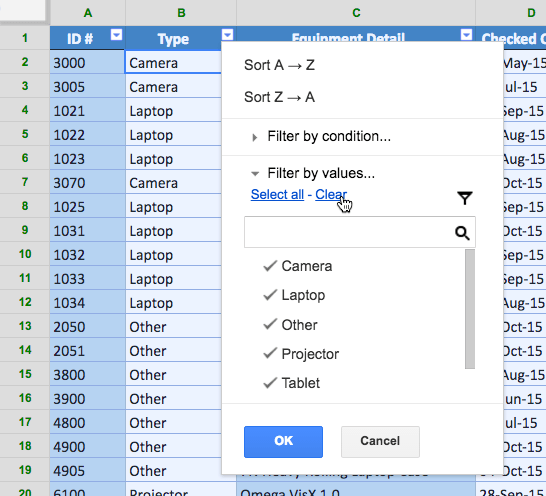
7. Select the data you want to filter, then click OK. For example, you would select Laptop and Projector to view only these types of devices.
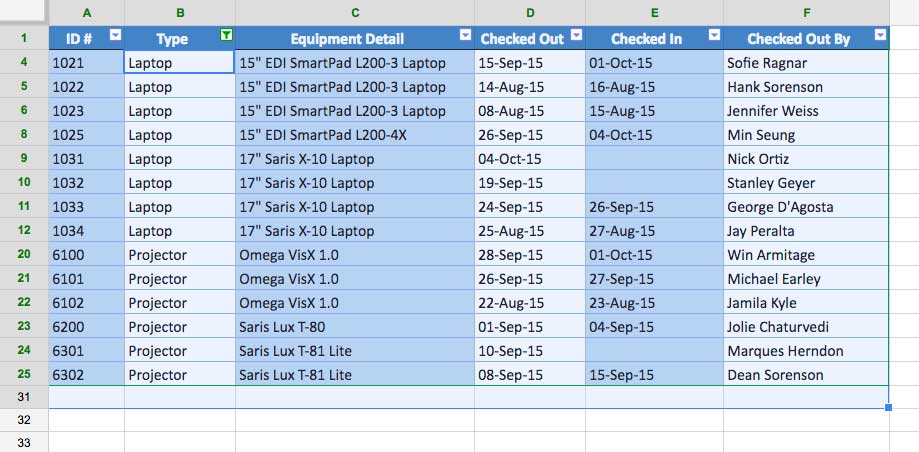
8. The data will be filtered, temporarily hiding any content that doesn't meet the criteria. In this example, only laptops and projectors are displayed.
Apply multiple filters
The filters are cumulative, meaning you can apply multiple filters to help narrow your results. For example, you might have filtered your spreadsheet to show laptops and projectors, and now want to narrow it down further to show only laptops and projectors that were checked in August.
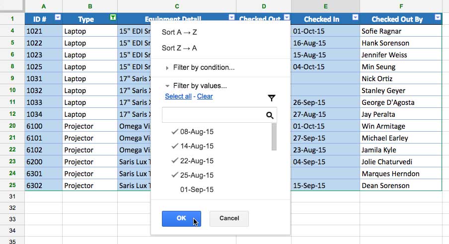
1. Click the drop-down arrow for the column you want to filter. For example, this will add a filter to column D to view information by date.
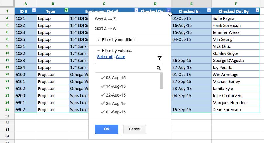
2. Select or deselect the boxes depending on the data you want to filter, then click OK. The example will deselect everything except August.
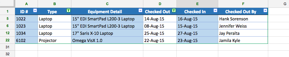
3. A new filter will be applied. In the example, the spreadsheet is now filtered to show only the laptops and projectors that were checked in August.
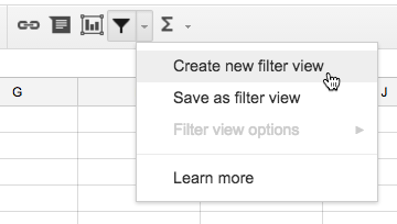
If you're collaborating with others on a spreadsheet, you can create filter views. Creating filter views allows you to filter data without affecting other people's data views; it only affects your own view. It also allows you to name the views and save multiple views. You can create filter views by clicking the drop-down arrow next to the Filter button.
How to remove all filters
Click the Filter button and the spreadsheet will return to its original format.