Table of Contents
Clustering is an unsupervised machine-learning technique that groups data points according to a chosen measure of similarity. The aim is to place points that resemble one another in the same cluster while separating points that differ.
A cluster is not an objective fact hidden in every dataset. The result depends on the features, scaling, distance measure, algorithm, and parameters. A useful analysis therefore explains how the groups were produced and whether they remain meaningful outside a chart.
What a data cluster looks like
When data has two measurable features, a scatter plot may reveal dense groups visually. The example below appears to contain three groups.
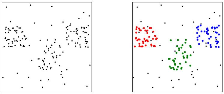
Real datasets often have more than two dimensions, overlapping groups, outliers, or irregular shapes. Visualization is a valuable first check, but an algorithm is needed to apply a consistent grouping rule.
Clustering is unsupervised learning
In supervised learning, training examples include known target labels. In clustering, the algorithm receives features without a correct cluster label for each point. It must discover a structure according to its mathematical objective.
Common uses include customer segmentation, grouping similar documents, detecting unusual observations, organizing images, and exploring measurements before building another model. A cluster should not automatically be interpreted as a demographic, diagnosis, or causal category.
Prepare the data before clustering
- Select relevant features. Irrelevant variables can dominate the grouping.
- Handle missing values. Choose an appropriate method rather than silently treating missing data as zero.
- Encode categories carefully. Numeric codes such as 1, 2, and 3 may create a false ordering.
- Scale numeric features. A variable measured in thousands can overwhelm one measured between 0 and 1.
- Choose a similarity measure. Euclidean distance is common, but it is not appropriate for every type of data.
- Inspect outliers. They may be errors, important rare cases, or a separate structure.
Major clustering approaches
Partitioning methods
Partitioning algorithms divide observations into a specified number of groups. k-means is the best-known example: it assigns points to the nearest centroid and updates the centroids until the assignments stabilize.
K-means is fast and easy to interpret, but it works best for roughly compact, similarly sized clusters. You must choose k, and the result can be sensitive to scaling, outliers, and initialization.
Hierarchical methods
Hierarchical clustering creates a tree of nested groups called a dendrogram. Agglomerative methods begin with each observation separate and repeatedly merge the closest groups; divisive methods begin with one group and split it.
This approach lets you inspect several possible cluster counts without rerunning a single fixed k. Its behavior depends on the distance metric and linkage rule. BIRCH and CURE are examples designed for particular large or irregular datasets.
Density-based methods
DBSCAN and OPTICS identify dense regions separated by sparser areas. They can find irregularly shaped clusters and mark isolated points as noise. Unlike k-means, DBSCAN does not require a cluster count in advance, but it does require density parameters and can struggle when cluster densities vary greatly.
Grid-based methods
Grid-based methods divide the feature space into cells and analyze populated regions rather than comparing every pair of observations. This can improve efficiency for large spatial datasets. STING and CLIQUE are established examples, with CLIQUE also addressing subspaces in high-dimensional data.
How to choose a clustering method
| Situation | Method to consider | Main caution |
|---|---|---|
| Compact groups and a known cluster count | k-means | Sensitive to scale and outliers |
| Need a nested view of possible groupings | Hierarchical clustering | Linkage choice changes the tree |
| Irregular shapes and meaningful noise points | DBSCAN or OPTICS | Density parameters require care |
| Large spatial or high-dimensional search | Grid/subspace methods | Grid resolution affects the result |
Evaluate whether the clusters are useful
There is rarely one perfect score. Combine several checks:
- Internal separation: are points closer to their own cluster than to other clusters?
- Stability: do similar groups appear after resampling or small parameter changes?
- Interpretability: can a domain expert explain what distinguishes the groups?
- External usefulness: do the groups improve a real decision or downstream task?
- Fairness: could the grouping encode sensitive attributes or produce harmful treatment?
A visually neat cluster can still be meaningless, and a useful structure may not appear clearly in a two-dimensional projection.
Correlation is not clustering
The Pearson correlation coefficient, usually written as r, measures the direction and strength of a linear relationship between two numeric variables. Its value ranges from -1 to +1. It does not assign observations to groups.
| Value of r | Typical interpretation | Linear direction |
|---|---|---|
| -1.00 | Perfect linear relationship | Negative |
| -0.70 | Strong linear relationship | Negative |
| -0.50 | Moderate linear relationship | Negative |
| -0.30 | Weak linear relationship | Negative |
| 0 | No linear relationship | None |
| +0.30 | Weak linear relationship | Positive |
| +0.50 | Moderate linear relationship | Positive |
| +0.70 | Strong linear relationship | Positive |
| +1.00 | Perfect linear relationship | Positive |
These labels are only rough conventions; what counts as “strong” depends on the field, measurement reliability, and purpose.
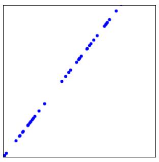
A perfect positive linear relationship:
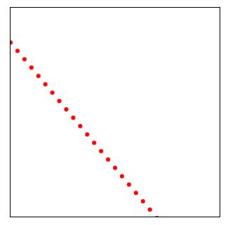
A perfect negative linear relationship:
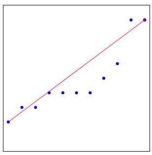
A moderately strong positive linear relationship:
No apparent linear relationship:
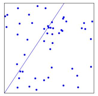
Correlation does not imply causation, and r can be near zero even when two variables have a strong nonlinear relationship. Always inspect the scatter plot and look for outliers.
Key distinction
Use clustering when you want to group observations. Use correlation when you want to summarize a linear relationship between two variables. Both can support exploratory analysis, but they answer different questions and should not be treated as interchangeable techniques.
Related Articles
 Line Learning Data: Explained6 minutes read
 Machine Learning Terminology: Explained6 minutes read
 How to Learn Machine Learning8 minutes read
 The Best Python Tools for Machine Learning and Data Science7 minutes read
 AI and Machine Learning in the Enterprise5 minutes read
 What Is Machine Learning? Complete Guide9 minutes read
Reader Comments 0
Sign in with email or Google to join the discussion.