Tricks using Google Sheets should not be ignored

When it comes to office software, we definitely can't ignore the Microsoft Office suite. However, if you need to go to online office job processing tools, Google's suite of applications will definitely meet our needs for editing, processing spreadsheets or presentations.

With Google Sheets, we can use it as an online version of Excel. You can proceed with data tables, online data storage as soon as you enter content. Besides, Google Sheets also supports us a lot with other useful features. Please refer to the tips article using the following Google Sheets of Network Administrator, so you can take advantage of this online tool.

1. Freeze rows and columns in Google Sheets:

In the process we proceed to process the spreadsheet content, there will be columns or tables we want to use in the always displayed mode to facilitate tracking. Therefore, we need to proceed to freeze that column or row.

At the main interface on the Google Sheets data sheet, we click on the View tab and select Freeze .

Tricks using Google Sheets should not be ignored Picture 1

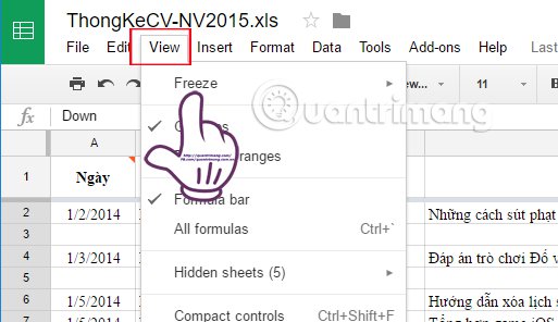
Next when we hover the mouse on Freeze, there are additional options for columns or rows. Here, you can choose to freeze any row or column if you want. Start calculating from row 1 column 1. In case we have selected 1 cell before performing operation click View, option will change to freeze row or column from the beginning to the selected cell (Up to current row / Up để hiện thời cột).

Tricks using Google Sheets should not be ignored Picture 2

2. Perform quick summary on Google Sheets:

As mentioned, Google Sheets is like an online Excel version, so we can perform Google Sheets calculations like when working with Excel. And the SUM calculation function is an extremely familiar function when processing data tables.

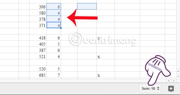
Google Sheets allows users to perform quick summary calculations, by pressing Ctrl and clicking on the cells you want to sum . Shortly thereafter, SUM will appear in the bottom right corner.

Tricks using Google Sheets should not be ignored Picture 3

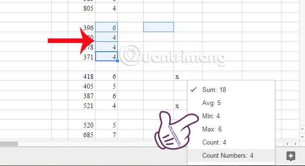
If we click on it, there will be a more detailed table with Min and Max values ​​of the series of sum or other values ​​as shown below:

Tricks using Google Sheets should not be ignored Picture 4

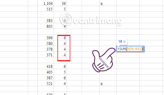
And the way to calculate the traditional total on Google Sheets is to type the formula into a blank = SUM (H29: H32), with H29 being the starting cell and H32 as the ending cell of the sum of the number as below. Shortly after, the calculation result will be displayed immediately.

Tricks using Google Sheets should not be ignored Picture 5

3. Create a Google Sheets registration form:

For those who need to create questionnaires, applications, Google Sheets will help us do that. How to do it is simple.

Step 1:

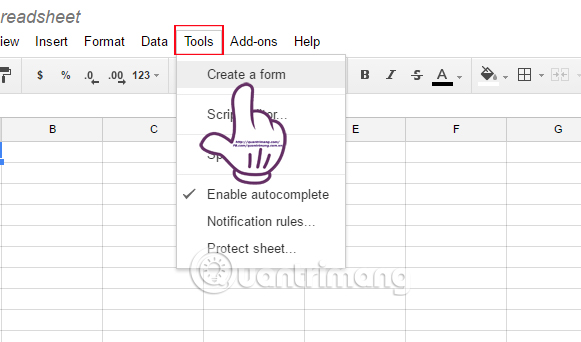
First of all, we need to open a new Google Sheest file. Then, click on the Tools section and select Create a form .

Tricks using Google Sheets should not be ignored Picture 6

Step 2:

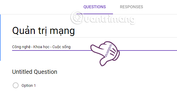
New interface appears. Here, the user will enter the title as well as the description content for this new form . The content will automatically be saved on this survey.

Tricks using Google Sheets should not be ignored Picture 7

Step 3:

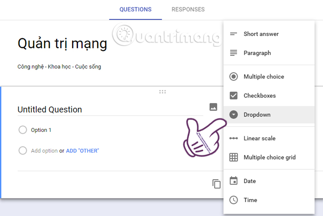
Next, we will fill in the question in Untitled Question , choose the type of answer as Multiple choice, check the answer (Checkboxes), or write the answer (Short answer), . . Then, we can change the settings for the form interface.

Tricks using Google Sheets should not be ignored Picture 8

4. Insert images into the box on Google Sheets:

If you insert the image into the spreadsheet content, it is very simple, but if you insert the image into the box, we will follow another operation.

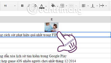
In the cell to insert images , type = image ("Image URL to insert") . The image will automatically resize to that cell.

For example, I will insert the image into the box with the following formula:

= IMAGE ("http://img.quantrimang.com/photos/image/2016/11/16/gay-me-1.jpg") as follows:

Tricks using Google Sheets should not be ignored Picture 9

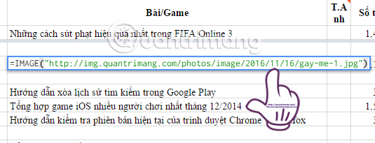
Soon, the image will appear in the cell's content.

Tricks using Google Sheets should not be ignored Picture 10

In addition, we can automatically adjust the image size with the formulas:

1. = image ("image URL", 2): resize the image to fit in the box.
2. = image ("Image URL", 3): keep the image size but does not change the cell size.

5. Conditional formatting on Google Sheets:

To highlight content in certain columns or fields, we will use conditional formatting on Google Sheet.

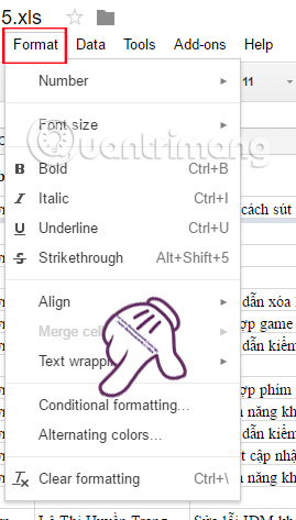
First, click Form and select Conditional formatting .

Tricks using Google Sheets should not be ignored Picture 11

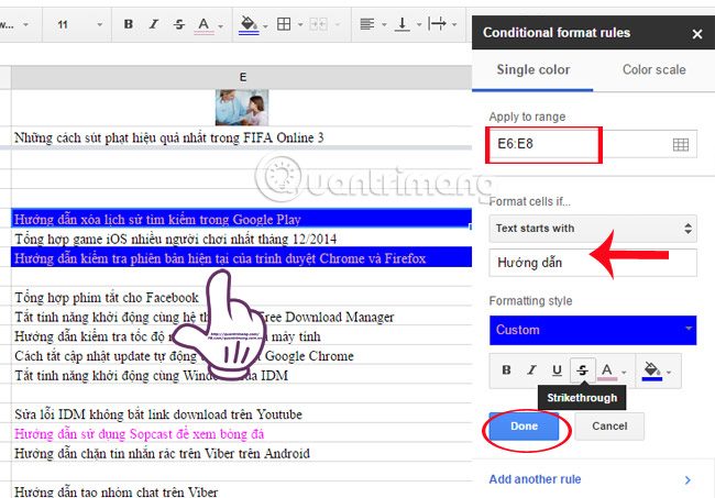
Right on the right side of the interface, a dialog box with conditional display items will appear. Here, you can select the columns or rows you want to format according to the Apply to range condition, select the condition to filter Format cells if , select the color for the format column, .

For example, with the example below, I will delineate rows from E6: E8 provided the text content in the row starts with the Instruction word. And then choose colors for those conditional lines. The results will show that 2 lines are marked with the given conditions. Finally click Done to save.

Tricks using Google Sheets should not be ignored Picture 12

The tips above are quite simple with not too complicated operations. These features as well as these actions will enable us to more proficiently use Google Sheets, increase productivity and manipulate faster when performing data processing with Google Sheet.

Refer to the following articles:

1. List of common shortcuts for Google Sheets on computers (Part 1)

1. How to convert numbers into words in Excel?

1. 10 ways to use the Paste feature in Excel

I wish you all success!