Some small tricks when working with Excel

Excel is an office application in Microsoft's MS Office suite, Excel is widely used in accounting and statistics. If you are a regular user of Excel, you will surely encounter the situation of repeating the update operation if the data changes or is inappropriate during use.

 

Here are 26 Excel tips for those who regularly work with charts and long lists.

Apply the format of this cell to another cell

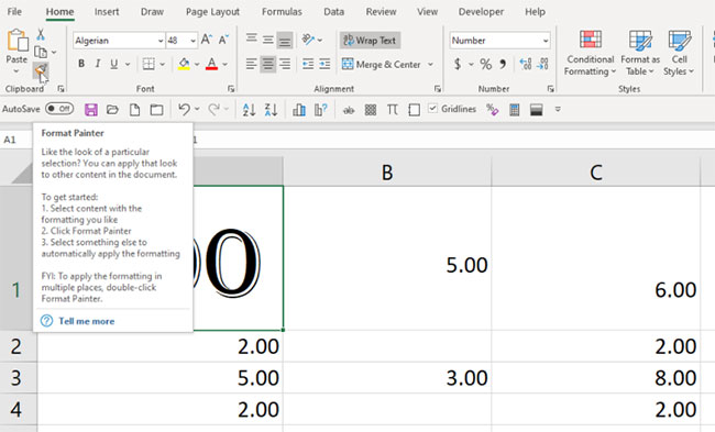
Let's say you're not just changing the wrapping in one cell, but changing the entire look—font, color, whatever. And you want to apply it to a bunch of other cells. The trick is the Format Painter tool , which is on the Home tab and looks like a paintbrush.

Select the cell you want, click the Format Painter icon , then click another cell to apply the same formatting—they'll look the same, but not their contents. If you want to apply it to multiple tabs, double-click the paintbrush icon, then click multiple cells.

 

Line Breaks and Text Wrap

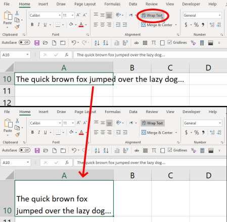
Typing into cells in a spreadsheet can be frustrating because by default, text goes on forever without wrapping onto a new line. You can change that. Create a new line by typing Alt + Enter (just pressing Enter will take you out of that cell). Or, click the Wrap Text option in the Home tab at the top of the screen, which means all text will wrap to the edges of the cell you're in. Resize the row/column and the text will "wrap" to fit the cell.

If you have multiple cells with text that exceeds the cell size, select them all before clicking Wrap Text . Or, select all the cells before you type anything into them and click Wrap Text . Then anything you type will be resized in the future.

Autofill cells

 

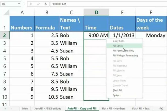
This one goes without saying, but is easily overlooked. If you have to enter a series of repetitive dates (1/1/20, 1/2/20, 1/3/20, etc.), start the series and move the cursor on the screen to the bottom right of the last cell – the fill handle. When it turns into a plus sign (+), click and drag down to select all the cells you need to fill. They will magically fill using the pattern you started with. The autofill function can also go up a column or left or right on a row.

You can even autofill without a lot of templates. Again, select the cell(s), go to the fill handle, right-click and drag. You'll get a menu of options. The more data you enter at first, the more the Fill Series option will help create better AutoFill options.

Fill cell contents in the fastest way

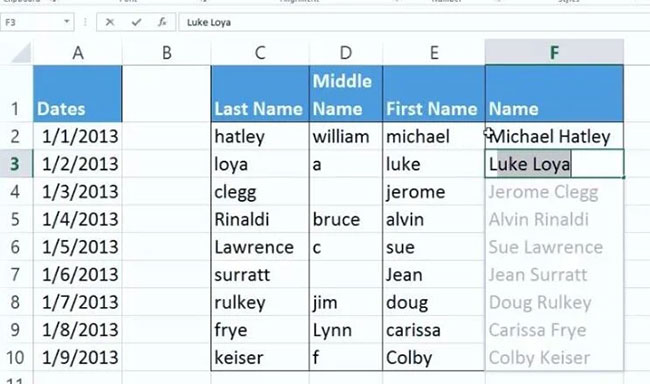
Flash Fill will intelligently fill a column based on the data pattern it sees in the first column (this is useful if the top row is the only header row). For example, if the first column is all phone numbers formatted as "2125034111" and you want them all to be (212) -503-4111" , start typing. By the second cell, Excel will recognize the pattern and display what it thinks you want. Just press Enter to use it.

This works with numbers, names, dates, etc. If the second cell doesn't give you the exact range, type in a few more numbers, as the pattern can be difficult to recognize. Then, go to the Data tab and click the Flash Fill button .

Press Ctrl + Shift to select

There are faster ways to select a set of data than using the mouse and dragging the cursor, especially in a spreadsheet that can contain hundreds of thousands of rows or columns. Click the first cell you want to select and hold Ctrl + Shift , then press the down arrow to select all the data in the column below, the up arrow to select all the data above, or the left or right arrows to select every row to the left or right, respectively. Using these navigation arrows, you can select an entire column as well as everything in the rows to the left or right. Only cells with data (even hidden data) are selected.

 

If you use Ctrl + Shift + End , the cursor will jump to the rightmost cell with data, selecting everything in between, even blank cells. So if the cursor is in the upper left cell (A1), every cell will be selected.

Ctrl + Shift + * (asterisk) can be faster, as it will select the entire contiguous data set of a cell, but will stop at blank cells.

Convert text to columns

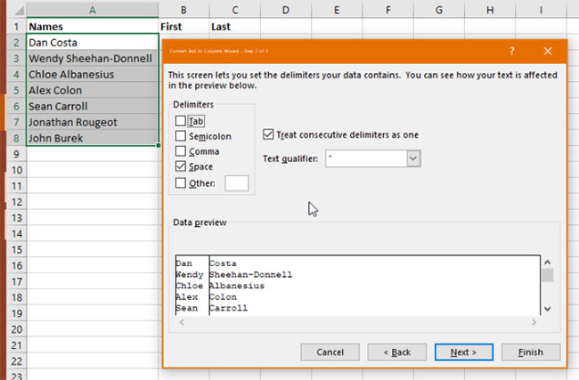
Let's say you have a column of full names, with first names next to last names, but you want two columns to split them up. Select the data, then on the Data tab (at the top), click Text to Columns . Choose to separate them by a delimiter (a space or a comma—great for CSV data values) or by a fixed width.

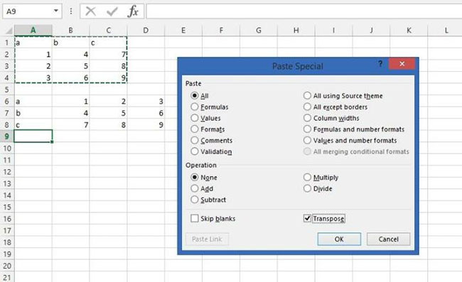
Use Paste Special to convert rows to columns and vice versa

You have a bunch of rows and want them to turn into columns or vice versa . You'd go crazy moving everything cell by cell. Copy that data, select Paste Special , check the Transpose box , and click OK to paste it in the other direction. Columns become rows, rows become columns.

Enter the same data into multiple cells

For some reason, you might find yourself typing the same thing into cells in a spreadsheet over and over again. It's horrible. Just click through the entire set of cells, either by dragging your cursor or by holding down the Ctrl key as you click each cell. Type it into the last cell, then press Ctrl + Enter - whatever you typed will appear in each selected cell.

This also works with formulas and will change the cell references to work with any rows/columns the other cells have in them.

 

Using Paste Special with Formulas

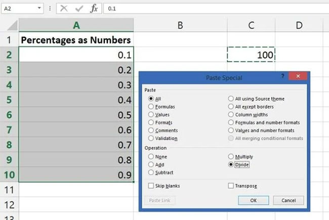
Let's say you have a large number in decimal format that you want to display as a percentage. The problem is, that 1 isn't 100%, but that's what Excel will provide if you click the Percent Style button (or press Ctrl-Shift-% ).

You want 1 to be 1%. So you have to divide it by 100. That's where Paste Special comes in. First, type 100 into a cell and copy it. Then, select all the numbers you want to reformat, choose Paste Special , click the "Divide" button. You'll have the numbers converted to percentages. This also works instantly for adding, subtracting, or multiplying numbers.

Using graphics in charts

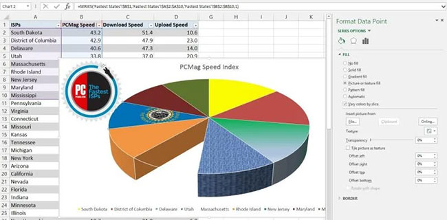
You can place a graphic in any element of an Excel chart. Each bar, each section in a pie chart, etc., can support an image. For example, above, there's a South Dakota state flag on the pie chart (placed by selecting the corresponding chart section, using the Series Options menu , and choosing "Picture or texture fill" ), along with an embedded PCMag logo (placed with the Insert tab's Pictures button). You can even choose the No fill option , which will create a blank space.

Clip Art can be cut and pasted into an element – ​​a bill to show how much money was spent, a water drip for plumbing costs, etc. Mixing and matching too many graphic elements makes it unreadable, but the options you have are worth tinkering with.

Save chart as template

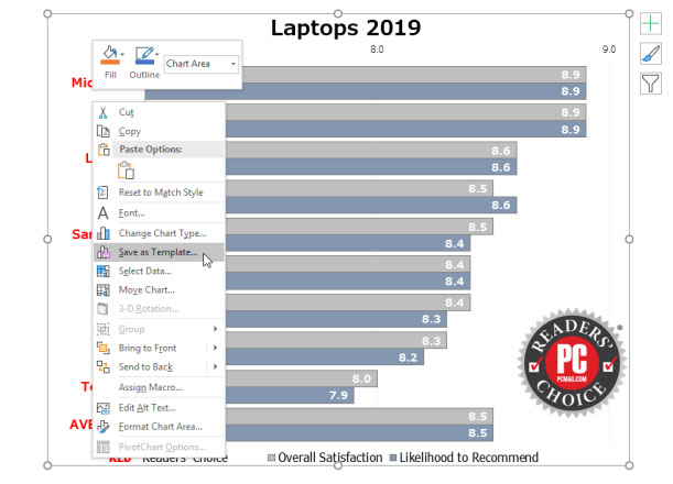
Excel has a wide variety of chart types, but it's nearly impossible to find a default chart that's perfect for your presentation. Fortunately, Excel's ability to customize all of its charts is great. But it can be frustrating to have to make frequent adjustments. The solution is to save your original chart as a template.

Once you've completed a chart, right-click it. Select Save as Template . Save the file with the CRTX extension in your default Microsoft Excel Templates folder . Once you're done, applying the template is a piece of cake. Select the data you want to chart, go to the Insert tab , click Recommended Charts , then go to the All Charts tab and the Templates folder . In the My Templates box , select the template to apply, and then click OK.

Some elements, like text and titles, won't be saved unless they're part of the selected data. You'll get all the font and color choices, embedded graphics, and even string options (like a drop shadow or glow around the chart element).

 

Working with cells on a worksheet

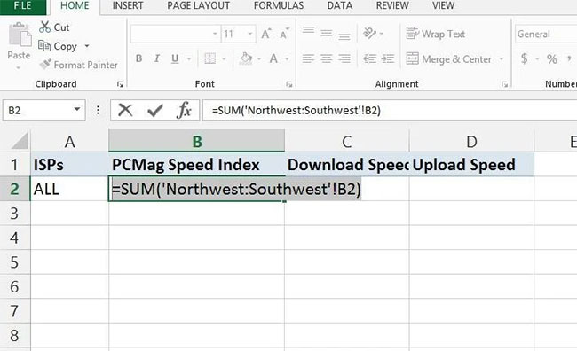
This tool, called 3D Sum , works when you have multiple sheets in a workbook that all have the same basic layout, such as quarterly or annual reports. For example, in cell B3, you always have the amount for the same corresponding week over time.

On a new sheet in the workbook, go to a cell and enter a formula like =sum('Y1:Y10'!B3). That tells a SUM (add everything) formula to all sheets titled Y1 to Y10 (which is 10 years) and look at cell B3 in each sheet. The result will be the sum of all 10 years. It's a great way to create a master spreadsheet that references ever-changing data.

Hide data but still be able to work with it

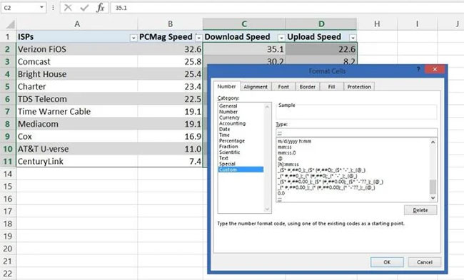
It's easy to hide a row or column—just select the entire contents by clicking on the letter or number heading, right-clicking, and choosing "Hide." (You can also unhide by selecting all the columns on either side, right-clicking, and choosing "Unhide.") But what if you only have a small portion of the data you want to hide, but still want to be able to work with it? Easy! Select the cells, right-click, and choose Format Cells. On the Number tab at the top, go to Category and select "Custom." Enter three semicolons (;;;) in the Type: field. Click OK. Now the numbers won't be visible, but you can still use them in formulas.

Hide the entire worksheet

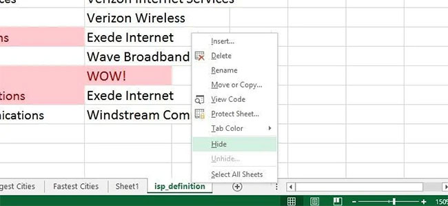
A typical Excel workbook—the file you're working in—can be loaded with multiple worksheets (each represented by a tab at the bottom, which you can name). Hiding a worksheet if you want, rather than deleting it, makes the worksheet's data available not only for reference but also for formulas on other worksheets in the workbook. Right-click the bottom worksheet tab and select Hide. When you need to find it again, you have to go to the View tab at the top, click Unhide, and select the worksheet name from the pop-up list.

There's also a Hide button on the View tab menu at the top. What happens when you click that? It hides the entire workbook you're using. It looks like you've closed the file, but Excel continues to run. When you close the program, it asks you if you want to save your changes to the hidden workbook. When you open the file, Excel gives you what appears to be a blank workbook—until you click Unhide again.

Use personal workbook for macros

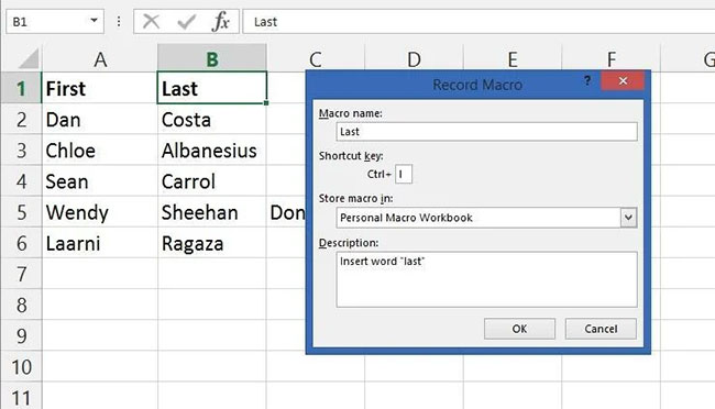
When you unhide all your workbooks, you may see a workbook listed that you didn't know you had hidden: Personal.XLSB. This is actually the personal workbook Excel created for you; it opens as a hidden workbook every time you start Excel. The reason to use this workbook is because of macros.

When you create a macro, it doesn't run on every spreadsheet you create by default (like it does in Microsoft Word)—a macro is linked to the workbook in which it was created. However, if you store the macro in Personal.XLSB, it will be available at all times, in all your spreadsheet files.

The trick is, when you record the macro, in the "Store macro in" field , select "Personal Macro Workbook" . (Record the macro by enabling the Developers tab - go to the File tab , select Options , click Customize Ribbon , then in the Main Tabs box , select Developers , then click OK ).

PivotTable

 

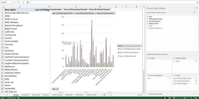
PivotTables are summaries of large collections of data that make it much easier to parse information based on reference points. For example, if you have an entire year's worth of test scores from all your students, a PivotTable can help you narrow things down to one student in one month.

To create a PivotTable, check that all columns and rows are titled properly, then select PivotTable on the Insert tab. Better yet, try the Recommended PivotTables option to see if Excel can choose the right type for you. Or try PivotChart, which creates a PivotTable with an accompanying chart for easier understanding.

Conditional formatting

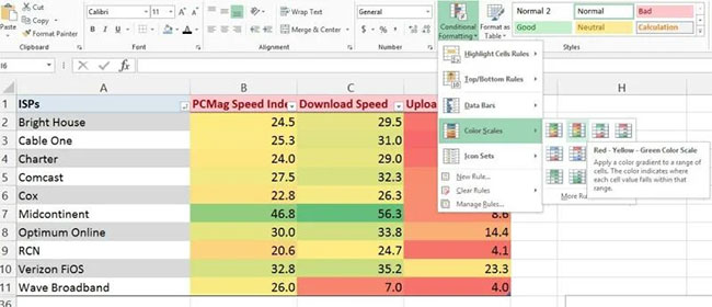
Looking at a huge amount of data and wondering what the highlights are? Who has the highest (or lowest) score, who are the top five, etc.? Excel's conditional formatting will do everything from putting borders around highlights to color-coding the entire table. It will even build a chart into each cell so you can visualize the top and bottom of the number range at a glance. (Above, the highest numbers are green, the lowest numbers are red.) Use the Highlighted Cells Rules submenu to create additional rules that search for things like text containing a certain string of words, repeating dates, duplicate values, etc. There's even a greater than/less than option so you can compare number changes.

Data validation

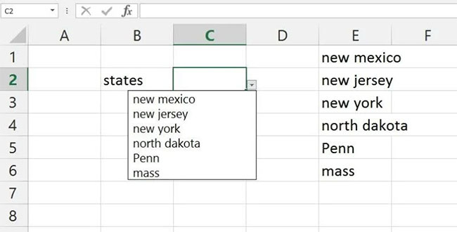
Creating a spreadsheet for other people to use? If you want to create a drop-down menu of choices to use in specific cells, that's easy. Select the cell, go to the Data tab , and click Data Validation . Under "Allow:" , select "List." Then, in the "Source:" field , enter the list, with commas between the options. Or, click the button next to the Source field and go back to the same sheet to select a data series - this is the best way to handle large lists. You can hide that data later, it will still work. Data validation is also a good way to restrict entered data - for example, give a date range and people can't enter any dates before or after the date you specify. You can even create an error message they'll see.

Insert screenshot

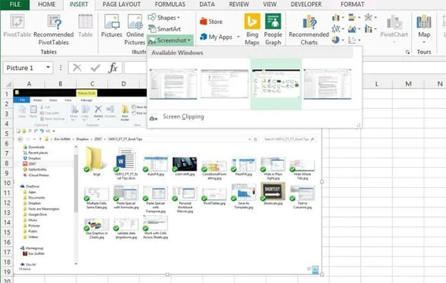
Excel makes it incredibly easy to take a screenshot of any other open program on your screen and insert it into your spreadsheet. Just go to the Insert tab, select Screenshot, and you'll get a drop-down menu showing thumbnails of all your open programs. Select one to insert the full-size image. Resize it as you like.

Insert Excel data into Word

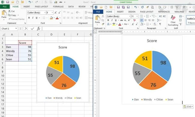
35 years ago, the idea of ​​transferring data from Excel to Word or PowerPoint was a thing in the world of Office suites. Today, it's a reality. Whether you're selecting data cells or a full-blown graphic, copy and paste it into the other program. The thing to note is that this is a linking and embedding process - if you change the data in the spreadsheet, it will also change in the Word DOC or PowerPoint PPT. If you don't want that, paste it as a graphic.

Use Word's own Paste Special tool for that. Or, when selecting it from Excel, go to the Home tab at the top, select the Copy menu , and use the Copy as Picture option . You can then paste the image into any program.

Use $ to prevent changes

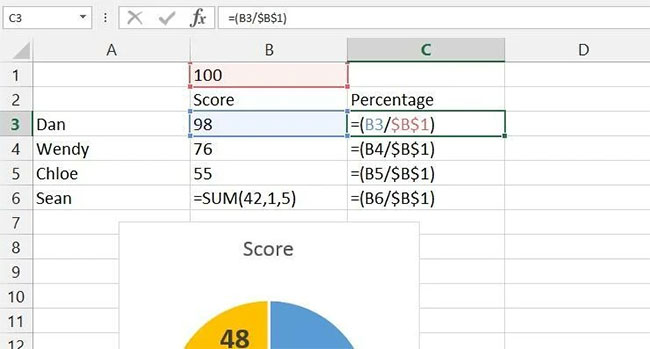
When writing a formula, you refer to cells by their position, such as A1. If you copy a formula and paste it into the next cell below, Excel will change that referenced cell to A2. To prevent this change, use the dollar sign ($). Typing $A1 , then cutting and pasting it into a new cell, will prevent changes in column (A); $1 prevents changes in row 1, and $A$1 prevents changes from moving in either direction when copying a formula.

This is useful when you have a single cell to use in a series of formulas. Let's say you want to divide everything by 100. You could create a formula like =(A1/100) , but that means you can't easily change the 100 across the board. Put 100 in cell B1 and use =(A1/B1) - but when you cut and paste it down, it turns into =(A2/B2) , then =(A3/B3) , etc. $ fixes that: =(A1/$B$1) can be cut and pasted down a row, but the $B$1 reference never changes. You can then change the value of 100 in the cell if needed to experiment with other changes.

Perform quick analysis

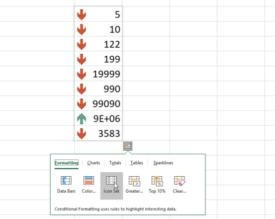
If you don't know exactly what information you want to apply to your data in Excel, try the Quick Analysis menu to quickly run through the options. Select the data and click the Quick Analysis box that appears in the lower right. You'll get a pop-up menu with options to quickly apply conditional formatting, create charts, process totals, display sparklines, and more.

Great shortcuts in Excel

Excel, like any great software, has lots of great shortcuts. Here are some of the best: Valuable Excel Shortcuts You Should Know .

Add quickly without a recipe

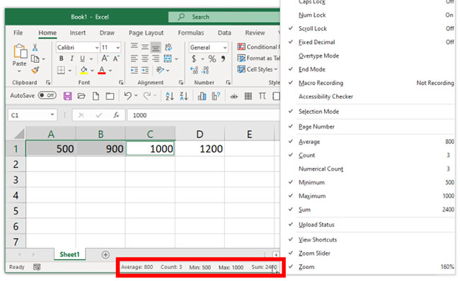
Do you have numbers in your spreadsheet that you want to calculate quickly without the hassle of going to a new cell and creating a SUM formula for the job? Excel now provides a quick way to do that. Click the first cell, hold down the Ctrl key, and click the second cell. Look at the status bar at the bottom and you'll see the total of the cells calculated for you.

Hold down Ctrl and click on as many cells as you like, the status bar will continue to show the sum for all cells. (Click on a cell with letters/words as content, it will be ignored.) Better yet, right-click on the status bar to get the Customize Status Bar menu and you can choose to add other elements that can be quickly calculated like this, such as seeing the average value or how many cells you clicked (or count, which is how many cells you clicked actually have numbers).

Fixed title when scrolling

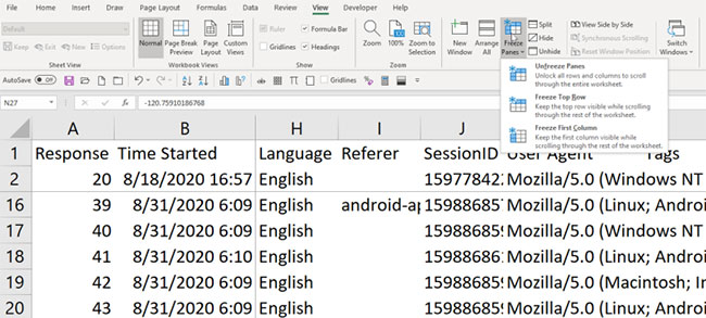
Working with large datasets in a spreadsheet can be difficult, especially when you scroll up/down or left/right and the rows and columns can be hard to follow. There is a simple trick to this if you have a header row or column, where the first row/column has a description. You freeze it so that when you scroll, that row and/or column (or rows and/or columns) do not move.

Go to the View tab and find Freeze Panes . You can easily freeze just the top row (select Freeze Top Row ) or the first column (select Freeze First Column ). You can do both at the same time by clicking on cell B2 and simply selecting Freeze Panes. Select any other cell and freeze all the cells above and to the left of it. Select cell C3, for example, and the two rows above and two columns to the left will not scroll. You can see this in the screenshot above, indicated by the darkened grid lines.

When you want to unfreeze Panes, you can select Unfreeze Panes from the menu.

New window for second view

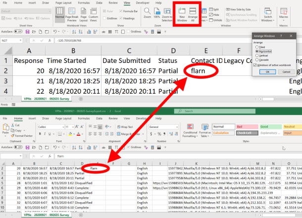
Spreadsheets can get very large, and you may have to interact with many different areas of the spreadsheet at once, such as cutting and pasting information from top to bottom multiple times. If there are hundreds of thousands of cells, scrolling can get annoying. Or, you can just open a second window on your screen with the exact same view of the same spreadsheet. Here's how: In the View tab , click New Window. You can also click Arrange All to arrange them on the screen in a way that works for you. You can see them arranged horizontally above. Then, type something into a cell in one window, and you can see it appear in the other window. This trick is especially useful if you have dual monitors.