Learn about Focus Cell: A hidden Excel setting that makes spreadsheets instantly easier to read.
The solution is a Microsoft Excel feature called Focus Cell. It addresses the readability issue by highlighting the active row and column with a subtle dynamic crosshair.
Table of Contents
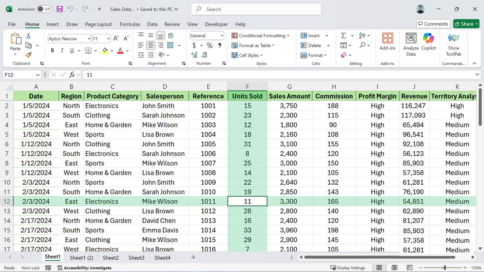
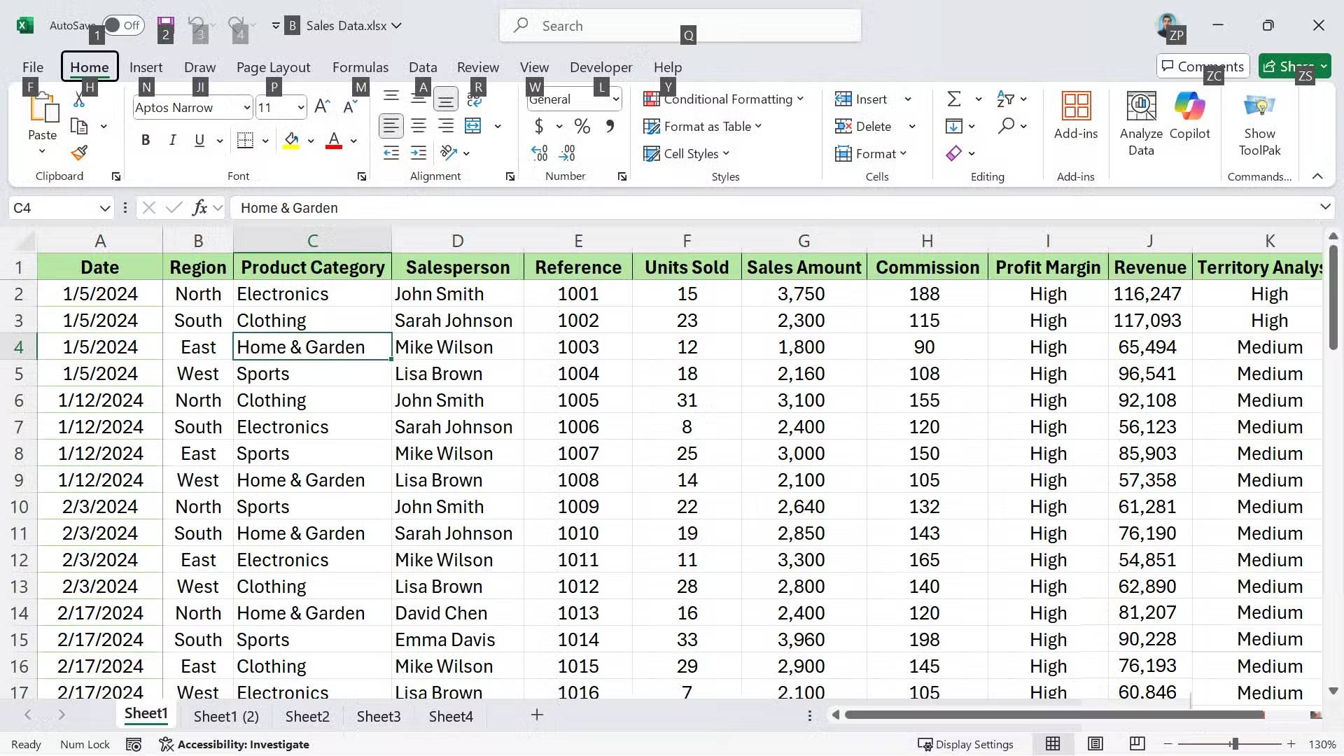
Working with large spreadsheets means constantly keeping track of rows and columns, and it's easy to lose your bearings when you're looking at hundreds of cells. People have tried various workarounds over the years—zooming in, using conditional formatting, adjusting column widths—but none have been truly effective.
The solution is a Microsoft Excel feature called Focus Cell. It solves the readability problem by highlighting the active row and column with a subtle dynamic crosshair. It's not flashy, but it eliminates visual clutter and makes navigating dense data much easier. This feature is now widely used in Excel for Microsoft 365 on Windows, macOS, and the web. It's quickly become a common setting when entering data. If you spend time working with spreadsheets, you need to know about this feature.
Focus Cell is a much better alternative to conditional formatting tricks.
Protect your spreadsheets from performance slowdowns caused by complex rules!
Before Focus Cell existed, the most common way to highlight active rows and columns was through conditional formatting combined with VBA macros. Technically, this method worked, but it was quite cumbersome and had real drawbacks.
The conventional method is to create a conditional formatting rule to check if a cell's row or column matches the currently selected cell. Because conditional formatting doesn't automatically detect the selected cell, you have to combine it with a "Worksheet_SelectionChange" macro that forces the spreadsheet to recalculate every time you move. The result is a makeshift cursor that works reasonably well. After using this method for a while, many people discourage its use.
The biggest problem with the VBA method is that it disrupts the Undo chain. Because the macro runs every time you click a cell, Excel's memory of previous actions is cleared, meaning you can't easily correct errors. The Focus Cell function solves all of these problems. It's a native UI feature that provides similar visual guidance without touching the data, interrupting the workflow, or slowing down the spreadsheet's calculation speed.
How to enable and customize Focus Cell in Excel
Choose a highlighting style that doesn't conflict with the existing theme.
If you're using Excel on the web or the latest version of Excel for Microsoft 365, enabling this feature takes only a moment. You don't need to search through the hidden Options menu or write any code. This setting is hidden right on the main ribbon.
To enable this feature, follow these steps:
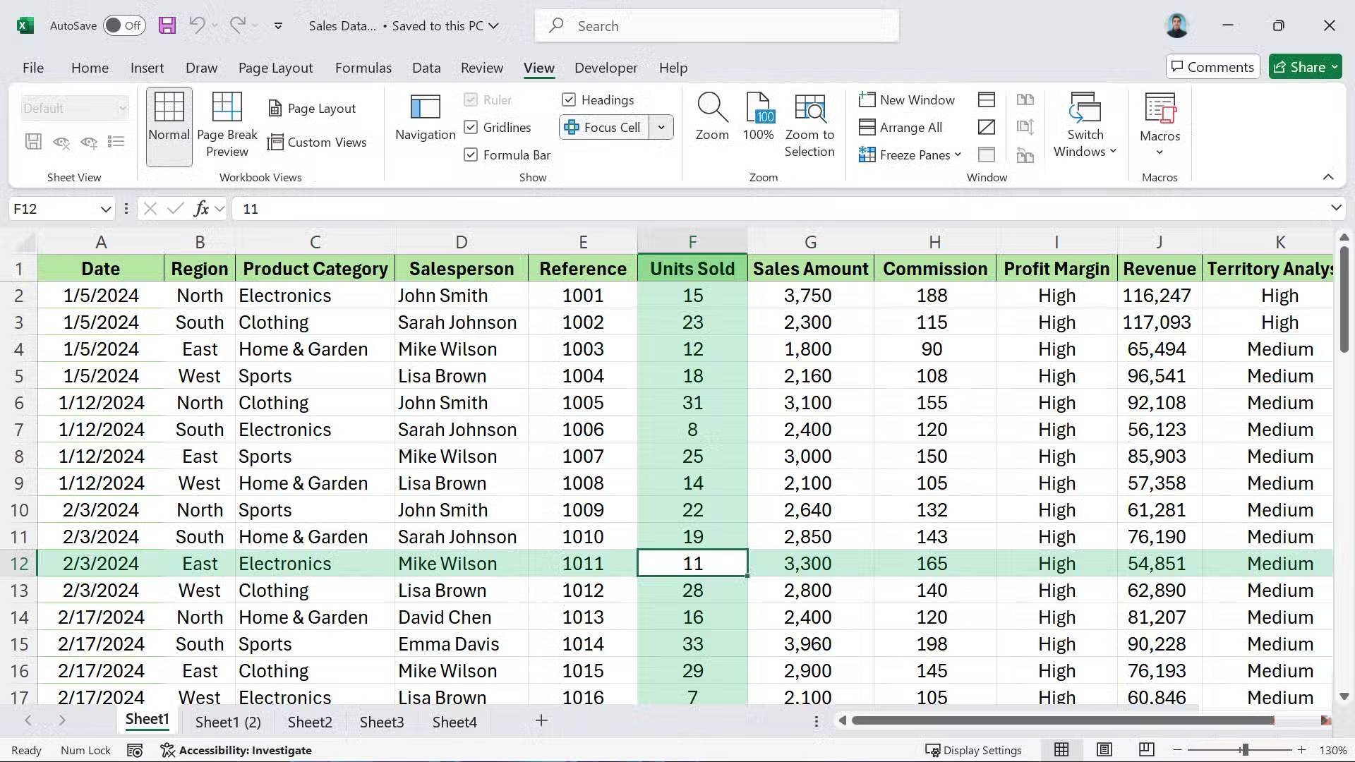
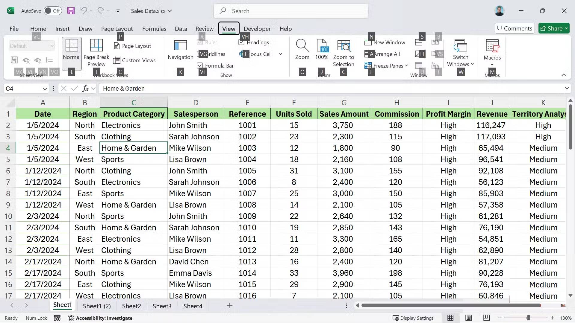
- Open your workbook and click the View tab on the ribbon at the top.
- Find the Focus Cell button (usually located next to the Gridlines and Headings toggle buttons).
- Click the button once to activate the cursor.
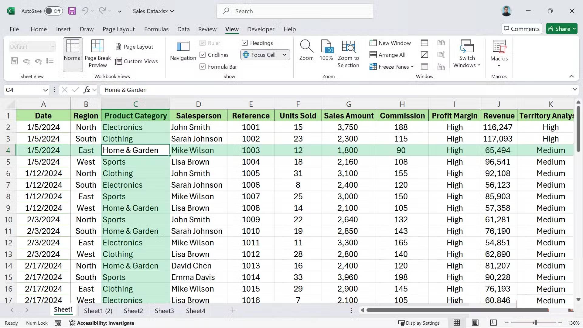
Once enabled, you'll see a colored highlight area that tracks your movement. It will follow you as you use the arrow keys or click the mouse, providing instant horizontal and vertical reference points.
Customize the Focus Cell interface to your liking.
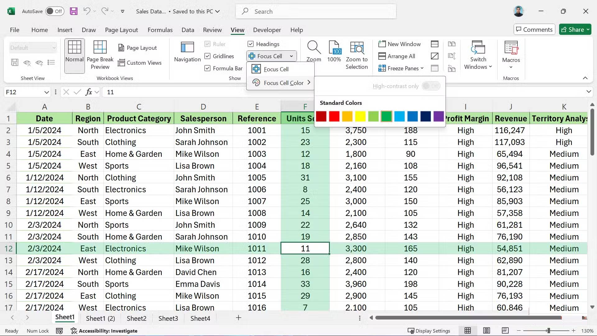
The default highlight color is usually light green, but you can change it to suit your visual preferences. This is especially useful if the spreadsheet already uses specific background colors for headers or alternating row styles. You want a color that stands out without making the text below difficult to read.
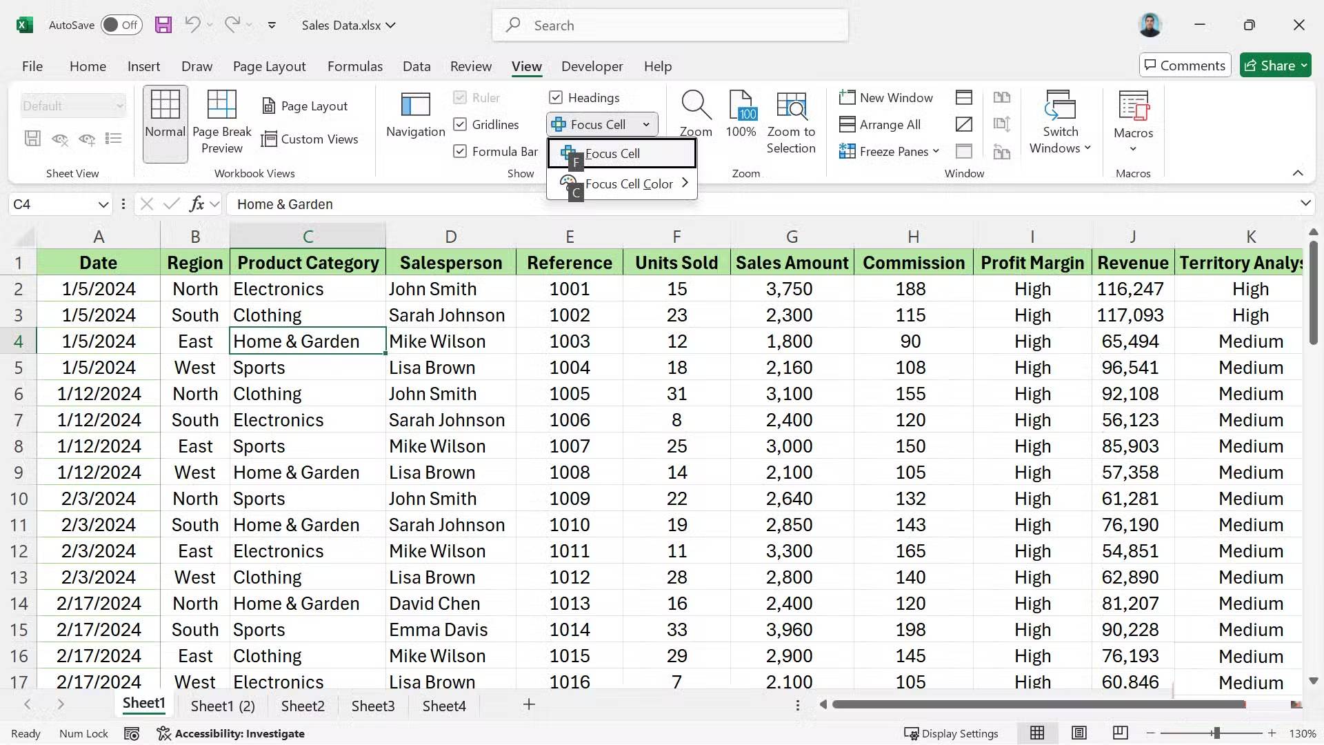
To change the color, click the drop-down arrow on the Focus Cell button in the View tab . You can choose from several preset colors. Many people prefer high-contrast colors, such as green, when working with numerical datasets, as it highlights the active row. Because the highlight area has partial transparency, it won't obscure your cell borders or font formatting.
Use keyboard shortcuts to quickly turn the highlight area on or off.
There are times when the cursor can get in the way—especially if you're trying to take a screenshot of a report or if you're presenting your screen to a group. Instead of navigating back to the View tab every time, you can use keyboard shortcuts on the Excel ribbon to toggle this feature on and off. Mastering essential Excel keyboard shortcuts for Windows can significantly speed up your workflow when dealing with these small toggle settings.
Press Alt > W > E > F in sequence (one key at a time). This sequence activates the View tab and toggles Focus Cell on/off . Remembering this shortcut allows you to use this feature as a temporary measure. You can turn it on while performing an audit and turn it off once you've found the data point you're looking for.
Combine Focus Cell with Freeze Panes
Keep the column headers visible while the cursor tracks the data.
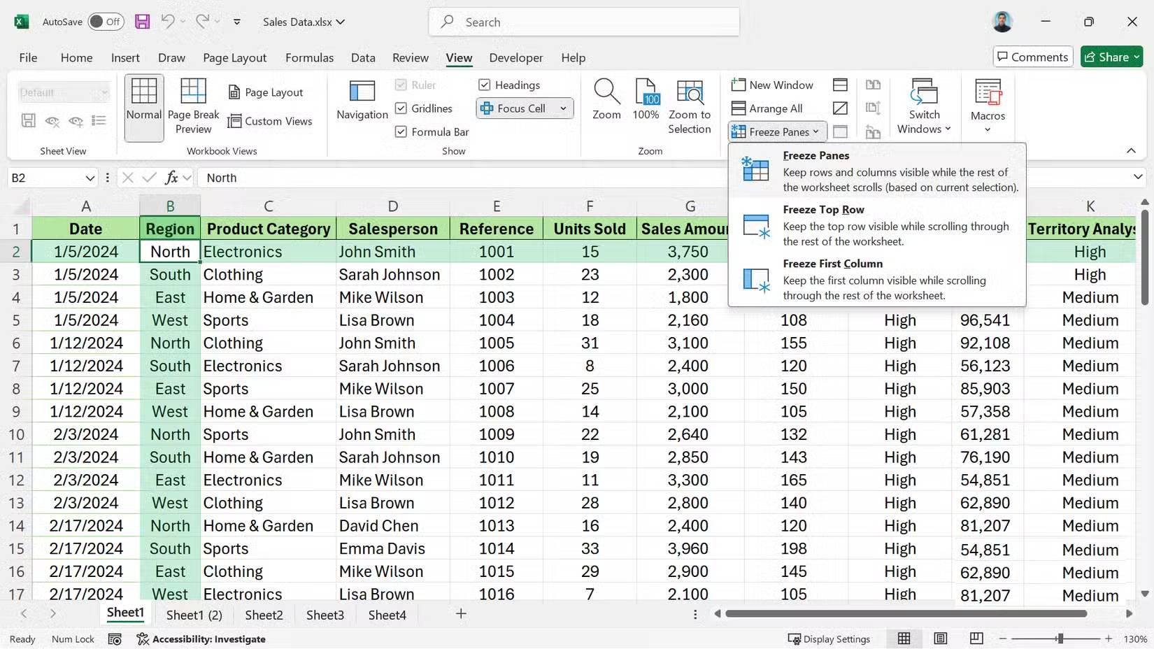
The Focus Cell function is very useful for knowing where you are, but it's even better when you combine it with Freeze Panes. On a large spreadsheet, you often lose track of column headers when scrolling down. When you combine these two features, you'll feel like you're in a control panel, where you always know which column you're in (thanks to the headers) and exactly which row (thanks to the Focus Cell cursor).
To set it up correctly:
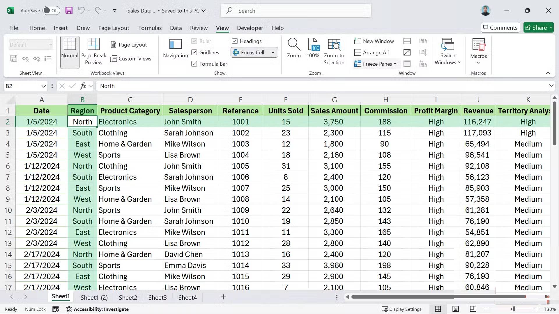
- Click the cell directly below the row you want to freeze and to the right of the column you want to freeze. For most spreadsheets, this is cell B2 (freezing row 1 and column A).
- Go to the View tab on the ribbon.
- Click on Freeze Panes , then select Freeze Panes again from the drop-down menu.
This combination eliminates almost all obstacles when entering data. Freeze Panes tells you what each column is for; the Focus Cell function tells you exactly where your cursor is located within that structure. One function handles context, the other handles position, and both functions do not conflict with each other.
Always keep both of these features enabled on any spreadsheet with more than about 40 rows. It's a small setup step but it eliminates a lot of unnecessary hassle. If you want to use this feature even more, Excel offers additional display options like Split View and Watch Window that work well with these features.
Was this article helpful?
Your feedback helps us improve.
Related Articles
 How to use Focus Cell to highlight Excel data2 minutes read
 How to open multiple spreadsheets side by side in Excel 20133 minutes read
 How to protect spreadsheets in Excel2 minutes read
 How to hide and hide sheets in Excel and show them again4 minutes read
 5 source to get macro to automate Excel spreadsheets7 minutes read
 Excel 2016 - Lesson 5: Basic concepts of cells and ranges11 minutes read
Reader Comments 0
Sign in with email or Google to join the discussion.