How to use the REDUCE function in Excel

For years, people have been solving complex spreadsheet problems the same way: Adding extra columns, stacking increasingly nested formulas, and when things get especially complicated, they resort to Excel VBA macros . This process worked well until they discovered the REDUCE function.

 

The REDUCE function allows you to iterate over data, building up the result step by step, much like a loop works in a programming language. Instead of scattering intermediate calculations across the worksheet, the entire process is encapsulated in a single formula, producing a single result.

If you've ever wished you could perform multiple sequential steps without filling up your workbook with extra intermediate columns and cells, then REDUCE is what you're looking for.

 

Note : This function is available only in Excel for the web, Excel for Microsoft 365, and Excel for Microsoft 365 on Mac.

What does the REDUCE function actually do (and why is it important)?

Process data step by step inside a formula and return a final result

 

REDUCE is a specialized formula that takes a list of data and applies a custom calculation to each item, combining the results as it goes. Finally, it returns a single result. That's the core idea.

More specifically, REDUCE is what Excel calls a LAMBDA helper function. This means that it is completely dependent on the calculation you define using the LAMBDA function. You can think of LAMBDA as the logic and REDUCE as the mechanism that executes that logic. Together, they perform iterative steps, where each calculation builds on the previous one. Instead of displaying each intermediate step on the spreadsheet (like a helper column), REDUCE keeps those steps internal using what is called a cumulative sum.

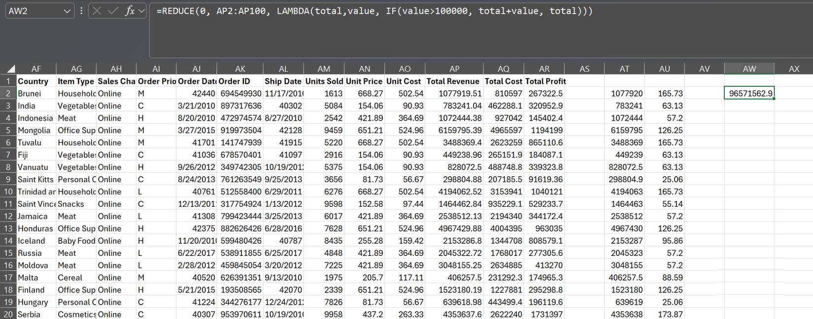
The basic syntax looks like this:

=REDUCE([initial_value], array, lambda(accumulator, value, body))

Here is the function of each part:

Argument	Purpose	Additional notes
[initial_value]	Starting value for cumulative sum.	For sums, you'll start with 0; for text construction, you'll use an empty string (""). This can also be a cell reference if the goal is to modify an existing value.
array	The source data that REDUCE cycles back and forth.	Each item in this array is processed in turn in the order in which it appears.
lambda	Custom calculations are applied to each item in your array.	It always uses 3 variables: Accumulator variable (usually denoted as A), current value from array (usually denoted as V) and body of the calculation (e.g. A + V). Accumulator variable stores running result from previous iterations, while value represents current item being processed.

 

The data flow is simple: The accumulator starts with an initial value. REDUCE takes the first element from the array, applies the LAMBDA operation, and updates the accumulator with the result. It then moves on to the next element and repeats the process, using the newly updated accumulator each time. Once each item is processed, REDUCE outputs the final accumulator. That output could be a number, a piece of text, or even an overflowed array, depending on the result the LAMBDA produced.

The advantage of this setup is that you no longer have to rely on multiple formulas scattered across your spreadsheet. Everything happens within one formula, contained in one cell, without the need for extra helper columns or intermediate steps.

Practical Ways to Use REDUCE in Your Workflow

Tasks that previously required a helper column or VBA are now contained within a formula

REDUCE works well in situations where results are cumulative over time, especially when each step builds on the previous one. However, it is also useful for common list operations. Once you see how it works, you will start to see opportunities to apply it in places where you might have previously relied on support columns or repeating formulas.

 

Example 1: Counting multiple independent items in one run

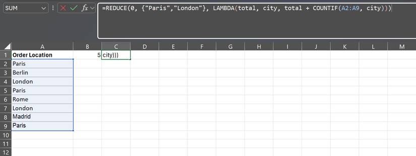
One of my favorite uses is counting multiple occurrences of items in a list at once. Let's say you have a column containing order locations and want to know the total number of orders from Paris and London. Instead of writing separate COUNTIF formulas and adding them together, you can do it all in a single expression:

=REDUCE(0, {"Paris","London"}, LAMBDA(total, city, total + COUNTIF(A2:A9, city)))

Start with 0 if you're accumulating a total. Instead of looping through each row of data, loop through the two cities of interest: Paris and London. For each city, the COUNTIF function checks how many times that city appears in column A and adds that result to the current total. The final output is a single number representing the combined order of both cities. If you need to adjust the geographic range, simply modify the list in the curly brackets—no need to restructure the formula.

Example 2: Total quantity embedded in mixed text string

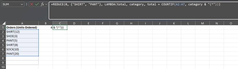
REDUCE is also useful when data is ambiguous. Imagine your orders column contains entries like 'SHIRT(5),' 'PANT(2),' and 'HAT(3),' where the item name and quantity are stored together. If you want to calculate the total quantity for specific categories—for example, SHIRT and PANT—regardless of how the quantity is sorted, the REDUCE function handles this neatly:

=REDUCE(0, {"SHIRT", "PANT"}, LAMBDA(total, category, total + COUNTIF(A2:A7, category & "(*")))

The key detail is the wildcard (*). Since the number in parentheses changes each row, the wildcard ensures that any text that begins with 'SHIRT' (or 'PANT') is included in the total. The REDUCE function loops through each category, counts all matching items in cells A2:A7, and adds up the totals. The result is a single value that represents the total quantity of both types of items, regardless of their individual quantities.