2 Excel Functions You Need to Know Before Struggling with Pivot Tables

Pivot Tables have long been the standard tool for summarizing and analyzing data in Microsoft Excel , and they work well for many tasks. However, if you've ever had to click through multiple menus just to adjust grouping or refresh data, you might prefer an easier approach. Excel's GROUPBY and PIVOTBY functions provide another way to summarize and sort data—one that's more flexible and transparent than the Pivot Table interface.

 

GROUPBY is a necessary function for simple data aggregation.

Helps simplify summary report creation

The GROUPBY function does exactly what it sounds like. It groups rows of data based on one or more columns and calculates summary values ​​for each group. It can be used to display total sales by region or average sales by product without setting up a pivot table.

 

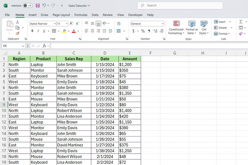
Let's say you have a sales dataset that tracks transactions across different regions and products. Using GROUPBY, you can switch between pivot tables, allow your analysis to automatically update, and get totals in a single formula.

It uses the following syntax:

=GROUPBY(row_fields, values, function, [field_headers], [total_depth], [sort_order], [filter_array], [field_relationship])

The parameters are analyzed as follows:

1. row_fields : The column or columns you want to group by. This can be one column, such as region, or multiple columns if you need nested grouping - for example, region and product together.
2. values ​​: The data you want to summarize. This is usually a column of numbers you want to sum, average, or count.
3. function : The calculation to be performed on each group. Common options include SUM , AVERAGE , COUNT , MAX , and MIN . You can use any function that works with arrays.

The following are optional parameters:

1. field_headers : Set this value to 1 to include column headers in the output, or 0 to exclude them. If you omit this value, Excel defaults to including headers.
2. total_depth : This value adds total rows to the result. Set this value to 1 for a single total, 2 for subtotals and grand totals, etc.
3. sort_order : Controls how the groups are sorted. Use 1 for ascending, -1 for descending, or omit this value to keep the original order of your data.
4. filter_array : A TRUE/FALSE array to filter which rows to include before grouping. This is useful when you only want to aggregate a subset of your data.
5. field_relationship : Controls how Excel interprets the relationship between multiple row_fields when grouping. Set to 0 (or omitted) to treat each combination of values ​​as a unique group. Set to 1 to create a hierarchical relationship, where the second field is nested under the first.

PIVOTBY creates familiar pivot layouts without the complexity

A classic two-way table with a single formula.

 

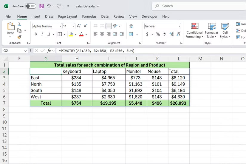
PIVOTBY takes data summarization to the next level by creating a two-dimensional summary—rows and columns working together. The difference is that you're writing formulas instead of clicking in dialog boxes.

This function is handy when you need to see how two categories intersect. For example, if you want to see sales by region for different products, PIVOTBY will arrange everything in a grid format that's easy to scan.

It has a long syntax with many optional parameters:

=PIVOTBY(row_fields, col_fields, values, function, [field_headers], [row_total_depth], [row_sort_order], [col_total_depth], [col_sort_order], [filter_array], [relative_to])

The parameters work as follows:

1. row_fields : The column or columns that define your rows. This is what appears on the left side of the output table. You can use one column or multiple columns for nested groups of rows.
2. col_fields : The column or columns that define your columns. These values ​​appear at the top of the output table, forming the width of the summary.
3. values ​​: The data you are summing. This is usually a column of numbers that you want to sum, average, or count for each combination of row and column values.
4. function : A calculation applied to each intersection of row and column groups. Common choices include SUM, AVERAGE, COUNT, MAX, and MIN.

The following are optional parameters:

1. field_headers : Set to 1 to include headers in the output or 0 to exclude them. If you omit this parameter, Excel defaults to including headers.
2. row_total_depth : Controls whether row totals and subtotals are added. Set to 1 for grand totals, 2 for subtotals and grand totals, etc.
3. row_sort_order : Determines how rows are sorted in the output. Use 1 for ascending order, -1 for descending order, or omit to maintain the original order from your source data.
4. col_total_depth : Same as row_total_depth , but for column totals. This option will add summary columns to the right of your output.
5. col_sort_order : Controls the sorting of column groups in your output table. Use 1 for ascending order, -1 for descending order, or omit to keep the original order.
6. filter_array : A TRUE/FALSE array that determines which rows from your source data will be included in the pivot calculation.
7. relative_to : Changes how sums and percentages are calculated when using certain aggregate functions. Set to 0 (or omitted) for standard sums. Set to 1 to calculate values ​​as a percentage of the row total or 2 for a percentage of the column total.