Instructions on how to use the Dmax function in Excel

When working with spreadsheet data, Excel function functions play an important role, helping users to perform as well as calculate all the data in the spreadsheet. The Dmax function in Excel is used to find the maximum conditional value enclosed in a column or row of a list, or a data table.

The user will find the maximum value in a Field field of the Database data sheet, to satisfy a Criterial given condition that the user selects. In the tutorial below, Network Administrator will show you how to use the Dmax function in Excel.

How to use the Dmax function in Excel

We have the syntax to use the following function:

Dmax (Database, Field, Criterial)

Inside:

1. database : list or related database including column headers.
2. field : field (column) needs to get the largest value. You can directly enter column headings in quotation marks or some represent column positions in the database: 1 for the first column, 2 for the 2nd column ., you can also enter the cell containing the title column needs to use example B3, C1 .
3. criteria : is the range of conditional cells, you can choose any exemption if that range contains at least one column Title and cell below the column heading containing the column conditions.

Note:

1. You should set the range of criteria criteria on the worksheet so that when the data is added, the range contains the same condition.
2. The range of conditions to be separated does not insert into the list or database to be processed.
3. criteria must contain at least the column heading and a cell containing the condition under the column heading.

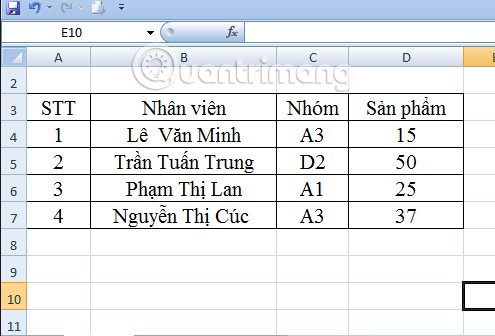
We have the following table data example:

Give a list of product volumes of each employee, belonging to different groups. Find employees with the most products The most popular product in group A3.

Instructions on how to use the Dmax function in Excel Picture 1

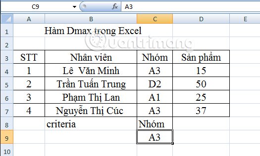
First, you need to create a range of criteria criteria Group A3 as shown below:

Instructions on how to use the Dmax function in Excel Picture 2

Based on the above syntax, we have the following formula:

Method 1:

In cell D10, enter the following formula: = DMAX (A3: D7, D3, C8: C9)

1. A3: D7 : is the most sought-after data area.
2. D3 : Product column and column need to find the most product number.
3. C8: C9 : the condition condition range in the table.

Instructions on how to use the Dmax function in Excel Picture 3

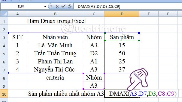
You press Enter and give the result as shown below:

Instructions on how to use the Dmax function in Excel Picture 4

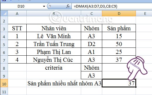
Method 2:

Also in cell D10, you enter the following formula: = DMAX (A3: D7, "Product", C8: C9)

In the D3 area, we will replace it with Product.

Instructions on how to use the Dmax function in Excel Picture 5

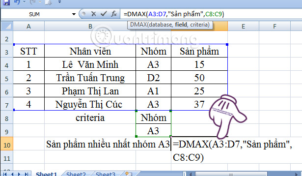
You also press Enter and give the same result as the 1st method performed above.

Instructions on how to use the Dmax function in Excel Picture 6

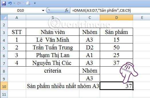
Above is a tutorial on implementing Dmax function in Excel. With this function you can use two ways and give similar results. If you want to find the largest value in the data table with the given conditions, Dmax function will help us find the required value.

Refer to the following articles:

1. Summary of expensive shortcuts in Microsoft Excel

1. You want to print text, data in Microsoft Excel. Not as simple as Word or PDF! Read the following article!

1. 10 ways to recover corrupted Excel files

I wish you all success!