Excel 2016 - Lesson 15: Relative and absolute cell references

1. Excel 2016 (Part 12): Formatting pages and printing spreadsheets
2. Excel 2016 (Part 13): Introduction to formulas
3. Excel 2016 (Part 14): Creating Complex Formulas

There are two types of cell references in Excel: relative and absolute . Relative and absolute references behave differently when copied and filled into cells. Relative references change when a formula is copied to another cell. Absolute references, however, remain the same no matter where they are copied.

 

Let's refer to TipsMake.com's tutorial article on relative and absolute cell references in Excel 2016 !

 

Watch the video below to learn more about cell references:

Relative references

By default, all cell references are relative. When copied across multiple cells, they change based on the relative position of the rows and columns. For example, if you copy the formula =A1+B1 from row 1 to row 2, the formula becomes =A2+B2 . Relative references are especially convenient when you need to repeat the same calculation across multiple rows or columns.

 

Create and copy a formula using relative references

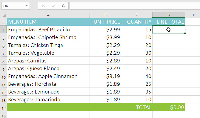
In the example below, we want to create a formula that will multiply the price of each item by the quantity. Instead of creating a new formula for each item, we can create a single formula in cell D2 and then copy it to the other rows. We will use relative references to calculate the total for each item correctly.

1. Select the cell containing the formula. In our example, we'll select cell D4 .

2. Enter the formula to calculate the desired value. In the example, we will type =B4*C4 .

 

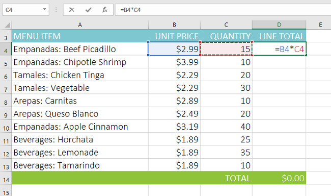
3. Press Enter on your keyboard. The formula will be calculated and the result will be displayed in the cell.

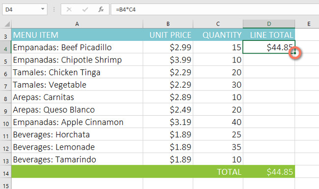
4. Locate the fill handle in the lower-right corner of the desired cell. In our example, we will locate the fill handle for cell D4.

5. Click and drag the fill handle to the cells you want to fill. In our example, we'll select cells D5:D13 .

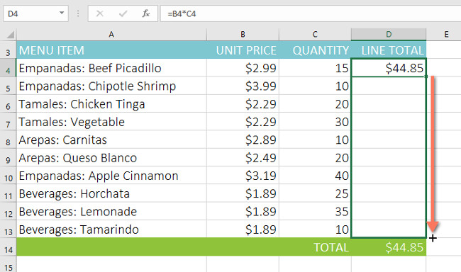
6. Release the mouse button. The formula will be copied to the selected cells with relative references, displaying the result in each cell.

 

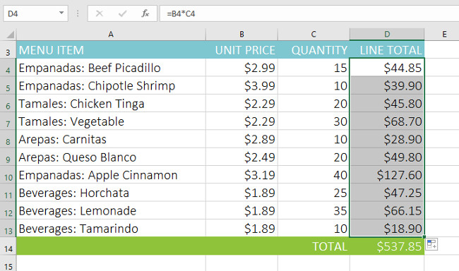
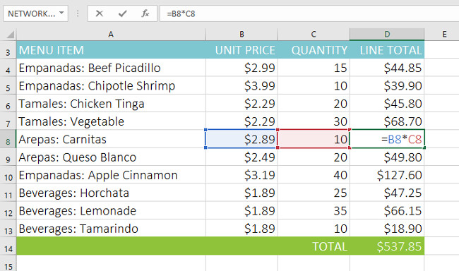
You can double-click on filled cells to check their correct formulas. The relative references for each cell should be different, depending on the row.

Absolute references

Sometimes you may not want a cell reference to change when you copy it to other cells. Unlike relative references, absolute references do not change when copied or filled. You can use an absolute reference to keep rows and/or columns in a row.

An absolute reference is specified in a formula by adding a dollar sign ($) . It can precede the column reference, the row reference, or both.

 

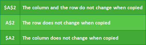
You will typically use the $A$2 format when creating formulas that contain absolute references. The other two formats are used less frequently.

When writing a formula, you can press the F4 key on your keyboard to switch between relative cell references and absolute cell references, as shown in the video below. This is an easy way to quickly insert an absolute reference.

Create and copy a formula using absolute references

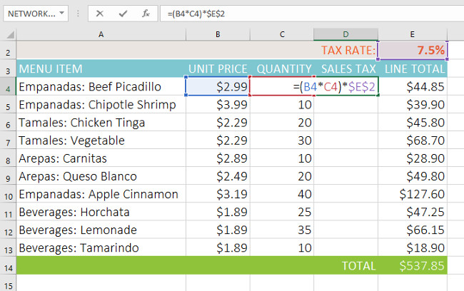
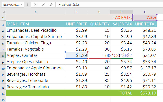
In the example below, we'll use cell E2 (which has a tax rate of 7.5%) to calculate the sales tax for each item in column D. To ensure the reference to the tax rate stays the same—even if the formula is copied and filled into other cells—we need to make cell $E$2 an absolute reference.

1. Select the cell containing the formula. In our example, we will select cell D4 .

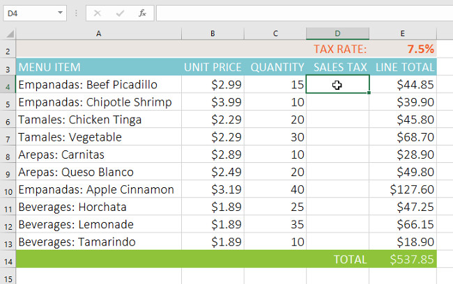
2. Enter the formula to calculate the desired value. In the example, we would enter =(B4*C4)*$E$2 , making $E$2 an absolute reference.

 

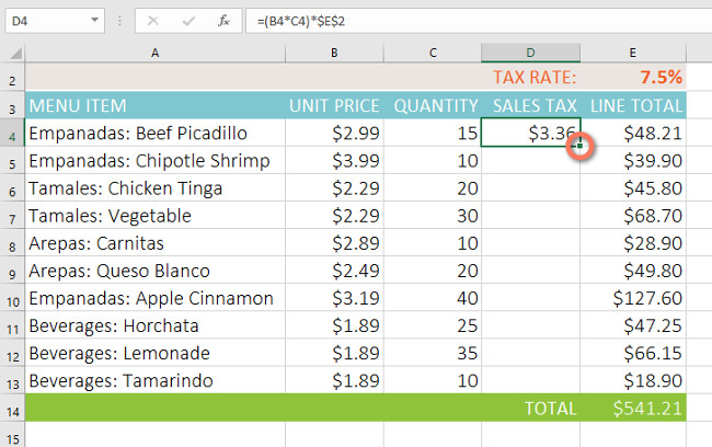
3. Press Enter on your keyboard. The formula will calculate and the result will be displayed in the cell.

4. Locate the fill handle in the lower-right corner of the desired cell. In our example, we will locate the fill handle for cell D4.

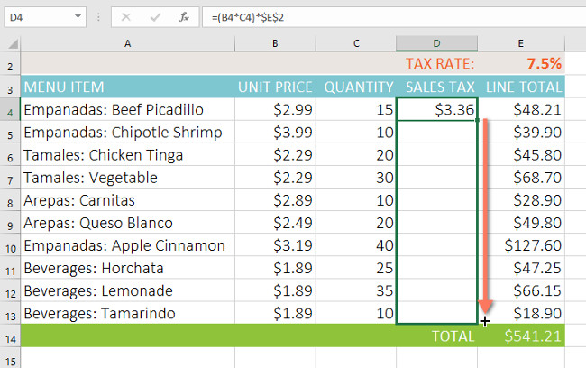
5. Click and drag the fill handle to the cells you want to fill (cells D5:D13 in the example).

6. Release the mouse. The formula will be copied to the selected cells with absolute references and the values ​​will be calculated in each cell.

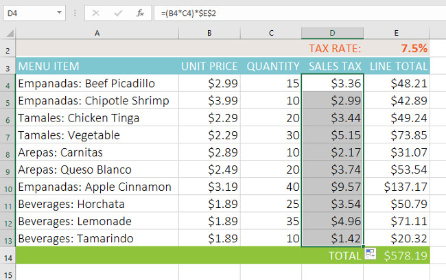
You can double-click on filled cells to check their formulas for accuracy. Absolute references should be the same in each cell, while other references are relative to the cell's row.

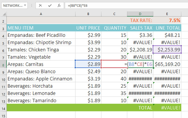
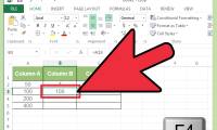
Be sure to include the dollar sign ($) whenever you make an absolute reference across multiple cells. The dollar signs have been omitted in the example below. This causes Excel to interpret it as a relative reference, which produces incorrect results when copied to other cells.

Using cell references with multiple worksheets

Excel allows you to reference any cell on a worksheet, which can be especially useful if you want to reference a specific value from another worksheet. To do this, simply begin the cell reference with the name of the worksheet followed by an exclamation point (!) . For example, if you wanted to reference cell A1 on Sheet1 , its cell reference would be Sheet1!A1 .

Note that if a worksheet name contains spaces , you will need to include single quotes (' ') around the name. For example, if you wanted to refer to cell A1 on a worksheet named July Budget , its cell reference would be 'July Budget'!A1 .

Referencing cells on worksheets

In the example below, we will reference a cell with a calculated value between two tables. This will allow us to use the exact same value on two different spreadsheets without having to rewrite the formula or copy data.

1. Locate the cell you want to reference and note the worksheet it is in. In our example, we want to reference cell E14 on the Menu Order worksheet.

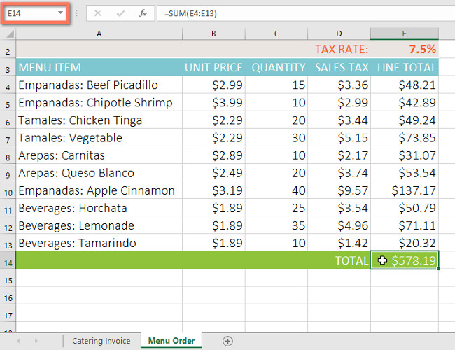
2. Navigate to the desired spreadsheet. In our example, we will select the Catering Invoice spreadsheet .

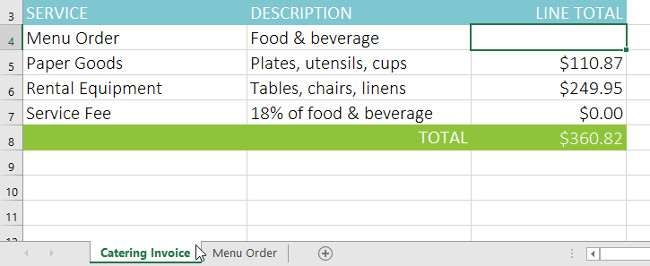
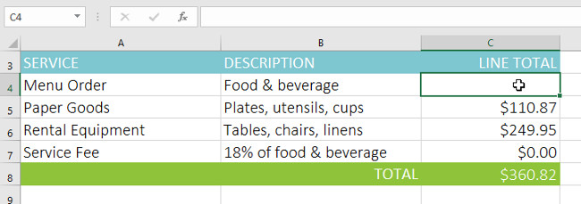
3. Locate and select the cell where you want the value to appear. In our example, we'll select cell C4 .

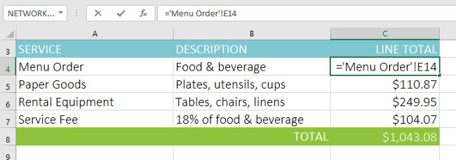
4. Type the equals sign (=) , the table name followed by an exclamation mark (!) and the cell address. In the example, we would type ='MenuOrder'!E14 .

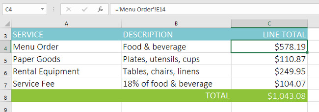
5. Press Enter on your keyboard. The value of the referenced cell will appear. Now, if the value of cell E14 changes on the Menu Order spreadsheet, it will be automatically updated on the Catering Invoice spreadsheet.

If you rename your worksheet at a later point, the cell reference will be automatically updated to reflect the new worksheet name.

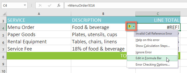
If you enter an incorrect sheet name, a #REF! error appears in the cell. In our example, we mistyped the sheet name. To edit, ignore, or investigate the error, click the Error button next to the cell and select an option from the menu.

See more articles:

1. Excel 2016 (Part 3): How to create new and open existing spreadsheets
2. Excel 2016 (Part 4): How to store and share spreadsheets
3. Excel 2016 (Part 5): Basic concepts of cells and ranges

Have fun!