Complete tutorial of Excel 2016 (Part 5): Basics of cells and ranges

See the video below to learn more about Basic Actions when working cells and ranges in Excel 2016 :

Basics of cells and ranges in Excel 2016:

1. A. Introduction
2. B. Learn about cells
   1. I. Select a box:
   2. II. Select a range of cells:
3. C. Cell contents
   1. I. Insert content:
   2. II. Delete cell contents:
   3. III. Delete cell:
   4. IV. Copy and paste the cell contents:
   5. V. Access to many paste options:
   6. VI. Cut and paste cell contents:
   7. VII. Drag and drop boxes:
   8. VIII. Use the fill handle function (a black note in the right corner - below the selected cell):
   9. IX. Continue a string with the fill handle:

B. Learn about Excel cells

Each spreadsheet is made up of thousands of rectangles, called cells.A cell is the intersection of a row and a column - in other words, where a row and column intersect.

Columns are defined by letters ( A, B, C ), while rows are determined by numbers ( 1, 2, 3 ). Each cell has its own name - or cell address based on columns and rows. In the example below, the selected cell intersects with column C and line 5, so the cell address is C5 .

Complete tutorial of Excel 2016 (Part 5): Basics of cells and ranges Picture 1

1. Note that the cell address also appears in the Name box in the top left corner and cell column and row headers are marked when the cell is selected.

You can also select multiple cells at once . A group of cells is known as a range of cells. Instead of a single cell address, you will refer to a range by using the first and last cell addresses in the cell range, separated by colons . For example, a range of cells including cells A1, A2, A3, A4 and A5 will be written as A1: A5. Please see the different ranges below:

1. Range of cells A1: A8

Complete tutorial of Excel 2016 (Part 5): Basics of cells and ranges Picture 2

1. Range A1: F1

Complete tutorial of Excel 2016 (Part 5): Basics of cells and ranges Picture 3

1. Range A1: F8

Complete tutorial of Excel 2016 (Part 5): Basics of cells and ranges Picture 4

1. If the columns in your spreadsheet are labeled with numbers instead of letters, you need to change the default reference type for Excel.

I. Select a box:

To enter or edit cell contents, you first need to select that box.

1. Click a cell to select it. In the example, we select cell D9 .

2. A border will appear around the selected cell and the column title and line titles will be highlighted. The box will remain selected until you click on another cell in the spreadsheet.

Complete tutorial of Excel 2016 (Part 5): Basics of cells and ranges Picture 5

1. In addition, you can also select cells by using the arrow keys on the keyboard.

II. Select a range of cells:

Sometimes, you may want to select a group larger than cells or a range of cells.

1. Click and drag the mouse until all the cells you want to select are highlighted. In the example, we select the range B5: C18 .

2. Release the mouse to select the desired range. The boxes will still be selected until you click another cell in the spreadsheet.

Complete tutorial of Excel 2016 (Part 5): Basics of cells and ranges Picture 6

C. Excel cell contents

Any information you enter into the spreadsheet will be stored in a cell. Each cell can contain different types of content, including text, formatting, formulas and functions .

1. Text : Cells may contain text, such as letters, numbers and dates.

Complete tutorial of Excel 2016 (Part 5): Basics of cells and ranges Picture 7

1. Format properties : Cells can contain formatting properties that change the way letters, numbers, and dates are displayed. For example, the percentage may appear to be 0.15 or 15%. You can even change the text of a cell or background color.

Complete tutorial of Excel 2016 (Part 5): Basics of cells and ranges Picture 8

1. Formulas and functions : Cells can contain formulas and functions that calculate the value of cells. In the example, SUM (B2: B8) adds the value of each cell in cell range B2: B8 and displays the total in cell B9 .

Complete tutorial of Excel 2016 (Part 5): Basics of cells and ranges Picture 9

I. Insert content:

1. Click a cell to select it. In the example, we select cell F9 .

Complete tutorial of Excel 2016 (Part 5): Basics of cells and ranges Picture 10

2. Enter something in the selected box, then press Enter on the keyboard. The content will appear in the box and the formula bar . You can also enter and edit cell contents in the formula bar.

Complete tutorial of Excel 2016 (Part 5): Basics of cells and ranges Picture 11

II. Delete cell contents:

1. Select the cell (s) with the content you want to delete. In the example, we select the cell range A10: H10 .

Complete tutorial of Excel 2016 (Part 5): Basics of cells and ranges Picture 12

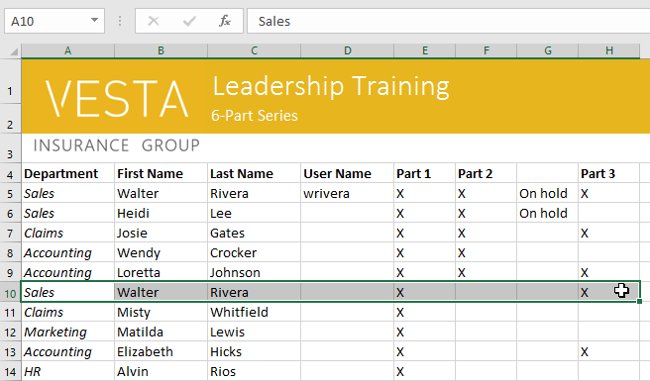
2. Select the Clear command on the Home tab, then click Clear Contents .

Complete tutorial of Excel 2016 (Part 5): Basics of cells and ranges Picture 13

3. Cell contents will be deleted.

Complete tutorial of Excel 2016 (Part 5): Basics of cells and ranges Picture 14

1. Alternatively, you can use the Delete key on the keyboard to delete content from multiple cells at once. The Backspace key will only delete content from one cell at a time.

III. Delete cell:

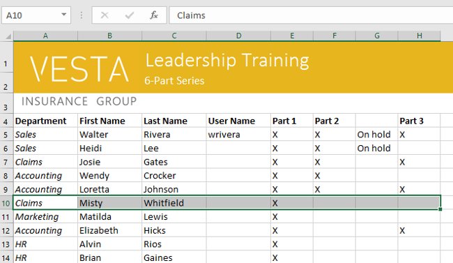
There is an important difference between deleting the contents of a cell and deleting that cell. If you delete the entire cell, the cells below it will move to fill the gap and replace the deleted cells .

1. Select the cell (s) you want to delete. In the example, we will select the range A10: H10 .

Complete tutorial of Excel 2016 (Part 5): Basics of cells and ranges Picture 15

2. Select the Delete command from the Home tab on the Ribbon.

Complete tutorial of Excel 2016 (Part 5): Basics of cells and ranges Picture 16

3. The cells below will change and fill the gap.

Complete tutorial of Excel 2016 (Part 5): Basics of cells and ranges Picture 17

IV. Copy and paste the cell contents:

Excel 2016 allows you to copy imported content into a spreadsheet and paste it into other cells, saving you time and effort.

1. Select the cell (s) you want to copy. In the example, we select the range F9 .

Complete tutorial of Excel 2016 (Part 5): Basics of cells and ranges Picture 18

2. Click the Copy command on the Home tab or press Ctrl + C on the keyboard.

Complete tutorial of Excel 2016 (Part 5): Basics of cells and ranges Picture 19

3. Select the cell (s) to which you want to paste the content. In the example, we choose F12: F17 . The copied cell (s) will have a cell surrounded by dashed lines.

Complete tutorial of Excel 2016 (Part 5): Basics of cells and ranges Picture 20

4. Click the Paste command on the Home tab or press Ctrl + V on the keyboard.

Complete tutorial of Excel 2016 (Part 5): Basics of cells and ranges Picture 21

5. The content will be pasted into the selected cells.

Complete tutorial of Excel 2016 (Part 5): Basics of cells and ranges Picture 22

V. Access to many paste options:

You can also access additional paste options, especially handy when working with cells containing formulas or formats. Just click the drop-down arrow on the Paste command to see these options.

Complete tutorial of Excel 2016 (Part 5): Basics of cells and ranges Picture 23

Instead of selecting a command from the Ribbon toolbar, you can quickly access commands by right- clicking . Simply select the cell (s) you want to format, then right-click. A drop-down menu will appear where you will find some of the same commands on the Ribbon.

Complete tutorial of Excel 2016 (Part 5): Basics of cells and ranges Picture 24

VI. Cut and paste cell contents:

Unlike copying and pasting, duplicating cell contents, cutting allows you to move content between cells.

1. Select the cell (s) you want to cut. In the example, we select the range G5: G6 .

2. Right-click and select Cut . Alternatively, you can use the command on the Home tab or press Ctrl + X on the keyboard.

Complete tutorial of Excel 2016 (Part 5): Basics of cells and ranges Picture 25

3. Select the cells to which you want to paste the content. In the example, we choose F10: F11 . The cut cells will have a box surrounded by a dashed line.

4. Right-click and select the Paste command. Alternatively, you can use the command on the Home tab or press Ctrl + V on the keyboard.

Complete tutorial of Excel 2016 (Part 5): Basics of cells and ranges Picture 26

5. The cut content will be removed from the original cells and pasted into the selected cells.

Complete tutorial of Excel 2016 (Part 5): Basics of cells and ranges Picture 27

VII. Drag and drop boxes:

Instead of cutting, copying and pasting, you can drag and drop cells that move their content.

1. Select the cell (s) you want to move the content. In the example, we select the range H4: H12 .

2. Hover over the border of the selected cells until the mouse pointer changes to a pointer with four arrows ( as shown below ).

Complete tutorial of Excel 2016 (Part 5): Basics of cells and ranges Picture 28

3. Click and drag the cells to the desired location. In the example, we move them to the range G4: G12 .

Complete tutorial of Excel 2016 (Part 5): Basics of cells and ranges Picture 29

4. Release the mouse. Cells will be dropped in the selected location.

Complete tutorial of Excel 2016 (Part 5): Basics of cells and ranges Picture 30

VIII. Use the fill handle function (a black note in the right corner - below the selected cell):

If you are copying cell contents to adjacent cells in the same row or column, using the fill handle function is a useful alternative to copying and pasting commands.

1. Select the cell (s) containing the content you want to use, then hover over the lower right corner of the cell to fill the appeared handle .

Complete tutorial of Excel 2016 (Part 5): Basics of cells and ranges Picture 31

2. Click and drag the fill handle until all the cells you want to fill in are selected. In the example, we choose the range G13: G17 .

Complete tutorial of Excel 2016 (Part 5): Basics of cells and ranges Picture 32

3. Release the mouse to fill the selected cell.

Complete tutorial of Excel 2016 (Part 5): Basics of cells and ranges Picture 33

IX. Continue a string with the fill handle:

Fill handle can also be used to continue a sequence. Whenever the contents of a row or column are in sequential order, such as numbers ( 1, 2, 3 ) or days ( Monday, Tuesday, Wednesday ), the fill handle function can guess what will come next in sequence. In most cases, you need to select multiple cells before using the fill handle to help Excel determine the bulk order . Take a look at the example below:

1. Select the range of cells that you want to continue. In the example, we will choose E4: G4 .

2. Click and drag the latch to continue the sequence.

Complete tutorial of Excel 2016 (Part 5): Basics of cells and ranges Picture 34

3. Release the mouse. If Excel understands the string, it will continue in the selected cells. In the example, Excel added Part 4, Part 5 and Part 6 to H4: J4 .

Complete tutorial of Excel 2016 (Part 5): Basics of cells and ranges Picture 35

Having fun!

Marvin Fry

Update 25 May 2019