8 Google Sheets Formulas That Make Work So Much Easier

Spreadsheets are supposed to save time, but sometimes they can be a real mess. No one likes having to dig through endless menus until they find some formula that makes the hard work easier.

 

8. VLOOKUP

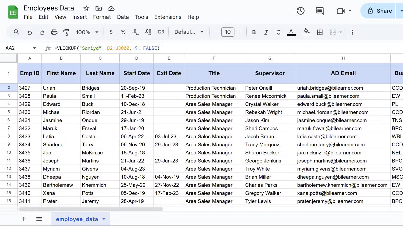
VLOOKUP searches for a specific value in the first column of a range and returns a corresponding value from another column in the same row. You can call it a lookup tool that saves you from having to manually scroll through huge data sets. The syntax of VLOOKUP is:

VLOOKUP(search_key, range, index, [is_sorted])

Where search_key is the value you want to find, and range is the table you're searching. The index parameter tells VLOOKUP which column to return data from, while is_sorted tells VLOOKUP whether the data is sorted or not.

 

Note : If you set is_sorted to FALSE , it will display exact matches, which is usually what you want for most lookup tasks.

7. SUMIF

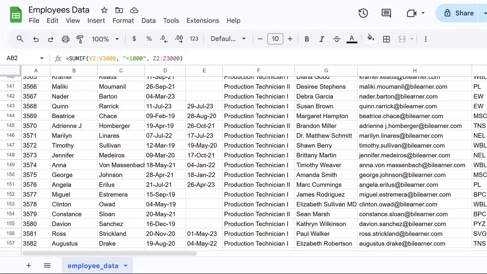
SUMIF adds values in a range based on specific criteria you set. Instead of manually calculating totals for different categories, this formula does the hard work and is very accurate.

While the basic IF function returns TRUE or FALSE based on conditions, the SUMIF function goes one step further by performing calculations on data that meets your criteria. The function syntax is as follows:

SUMIF(range, criteria, [sum_range])

Where range contains the cells you're testing against, criteria is your condition, and sum_range is the actual values to add. If you omit sum_range , SUMIF will add the values in that range itself. This function only works with text, numbers, and even wildcards, such as asterisks (*) for partial matches.

 

=SUMIF(V2:V3000, "<1000", Z2:Z3000)

6. CONCATENATE

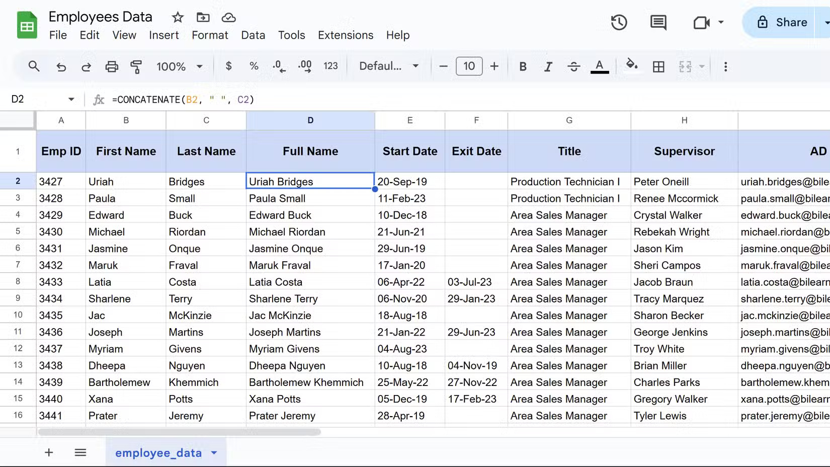
This function combines text from multiple cells into a single cell. Whether you need to merge first and last names, create email addresses, or create custom labels, you can use this function in a formula to handle text manipulation.

You can also use the ampersand (&) symbol as a shortcut for basic data concatenation, although using the CONCATENATE function in Google Sheets offers more flexibility for complex concatenations. The syntax for the CONCATENATE function is:

CONCATENATE(string1, [string2, .])

Here, string1 is the first text value and you can add an unlimited number of additional strings. Each argument can be a cell reference, actual text in double quotes, or a combination of both.

Note that this function does not automatically add spaces, so you need to add them manually as separate parameters, as in the following example.

=CONCATENATE(B2, " ", C2)

5. COUNTIF

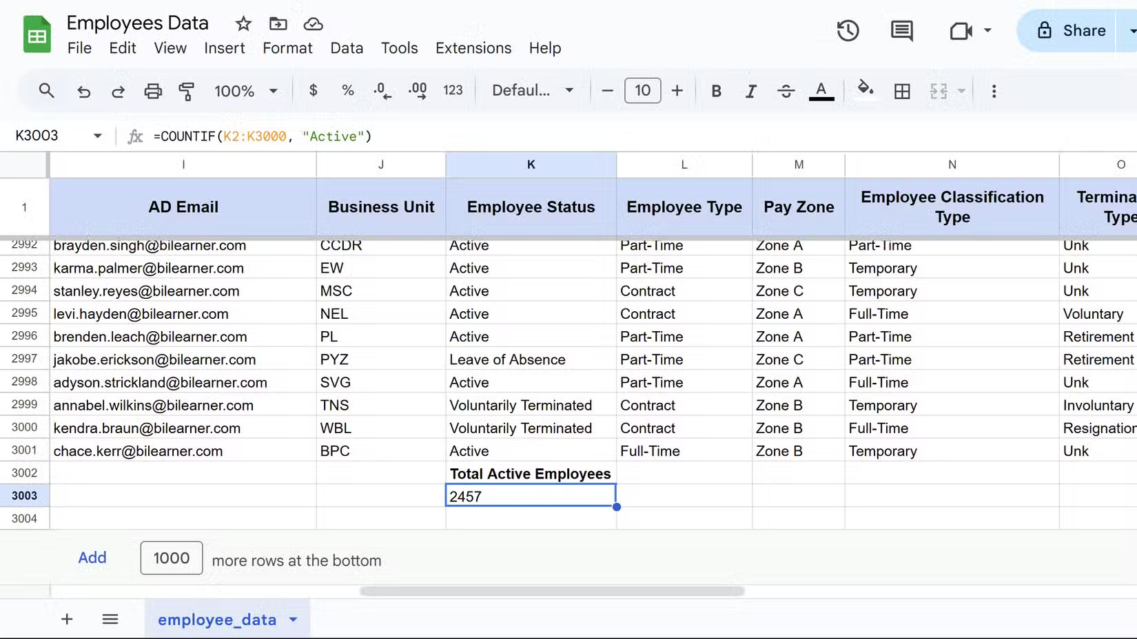
COUNTIF counts cells in a range that meet specific criteria. When you need to track the number of items in certain categories—like counting completed tasks or summarizing specific responses—this formula eliminates manual counting errors.

 

This formula works well for analyzing survey data, tracking inventory, and performance metrics. The syntax for COUNTIF is:

COUNTIF(range, criteria)

Where range specifies the cells you want to check, and criteria specifies the conditions the cells must meet to be counted. Criteria can include text, numbers, or logical operators. Here's an example:

=COUNTIF(K2:K3000, "Active")

 

4. ARRAYFORMULA

Next on the list is ARRAYFORMULA, which automatically applies a single formula to an entire range of cells. Instead of copying the formula down hundreds of rows, you just write it once and let Google Sheets handle the rest.

This is useful when working with large, ever-expanding data sets. Instead of having to remember to pull down the formula every time new data appears, ARRAYFORMULA automatically updates everything. The basic syntax encapsulates your regular formula:

=ARRAYFORMULA(đặt_công_thức_ở_đây)

However, you need to refer to an entire column or range instead of individual cells. For example, instead of A2, you would use A2:A to include the entire column from row 2 down.

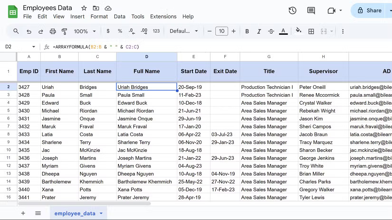
Here is a real-world example combining first and last names:

=ARRAYFORMULA(B2:B & " " & C2:C)

3. FILTER

This formula extracts specific rows from a data set based on conditions you specify. When you only need to see certain employees, projects, or sales records without manually hiding rows, this formula creates a dynamic subset instantly.

The most appreciated thing about FILTER is that the results automatically update when the source data changes, unlike manual filtering. This formula is useful for dashboards and live reports. The syntax follows the following pattern:

FILTER(range, condition1, [condition2], .)

Range contains your data, while condition1 specifies the first criteria. Additionally, you can stack multiple conditions for more precise filtering, as shown in the example below.

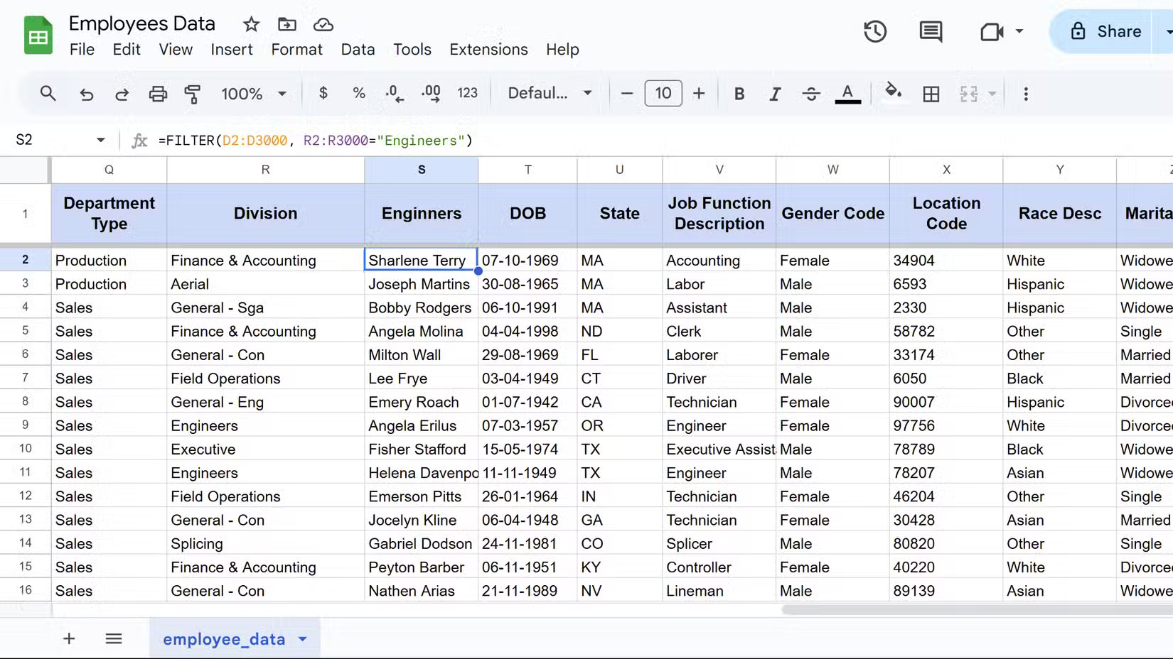
=FILTER(D2:D3000, R2:R3000="Engineers")

This formula only displays Engineering employees from the employee database. Therefore, you will get the exact subset you need without having to scroll through irrelevant records.

 

2. QUERY

QUERY brings database-style searching to Google Sheets using a SQL- like language . It may sound intimidating at first, but this Google Sheets function can save you hours each week. Once you master the basics, it's simple and powerful for analyzing office data.

This function combines filtering, sorting, and grouping into a single formula. Instead of using multiple functions, you can extract exactly what you need with just one command. The basic syntax is as follows:

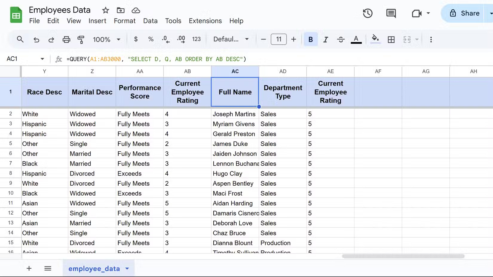
QUERY(data, query, [headers])

The data parameter contains your range, query contains the SQL-like command in double quotes, and headers specifies the number of header rows to include. In the following example, QUERY analyzes employee performance data:

=QUERY(A1:AB3000, "SELECT D, Q, AB ORDER BY AB DESC")

1. IMPORTRANGE

This function imports data from other Google Sheets files directly into the current spreadsheet. When you manage multiple project files, budget trackers, or departmental reports, IMPORTRANGE can eliminate the copy-paste process for you.

It maintains a direct connection between files, so when a colleague updates the master sales spreadsheet, your dashboard automatically reflects those changes without having to update manually. The syntax requires two key pieces of information.

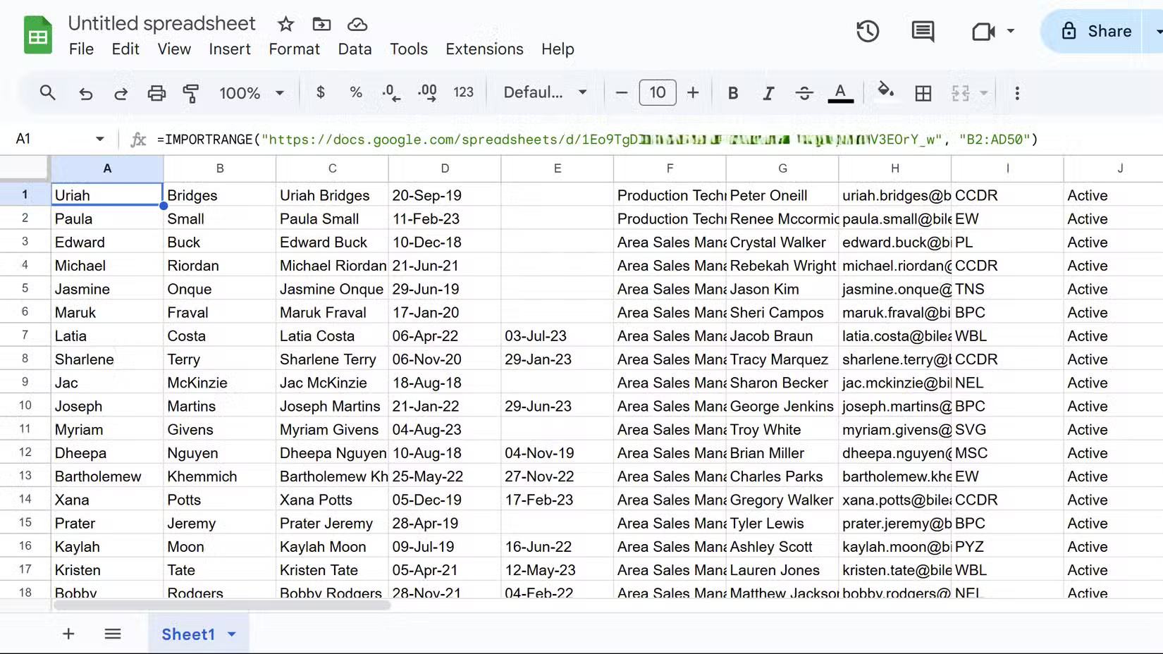
IMPORTRANGE("spreadsheet_url", "range")

spreadsheet_url is the full web address of the source file, while range specifies exactly which cells to import using standard notation, such as "Sheet1!A1:C10". Here's an example:

=IMPORTRANGE("https://docs.google.com/spreadsheets/d/abc123", "B2:AD50")

These 8 formulas make using spreadsheets significantly easier. They take a little time, but you'll see the time savings when you use them regularly. Data tasks that used to take hours now take just minutes, and it's well worth it.