6 useful functions in Google Sheets you may not know yet

Google Sheets is an extremely flexible and outstanding tool that combines the setup and calculation of data in spreadsheet form. It works based on the cloud feature, so it provides many interactive functions, automated data collection, even pulling data from third-party APIs.

You often work with spreadsheets like Excel, iWork Numbers, Zoho Sheet or Open Office Calc that will easily use Google Sheets. If you are new to Sheets, or are exploring the Spreadsheet program, here are six useful functions for your data.

For more tips in Google SpreadSheets, click here.

1. JOIN: Combining words in Google Sheets

The JOIN function is used to deepen the string of values ​​into a text to facilitate the use. Or simply synthesize some key values ​​or some HTML.

Type & to connect the values ​​of different cells and use quotation marks with any text you want to insert.

For example, we use the following calculation:

= A1 & "" & B1 & "and" & A2 & "" & B2

and the result is "4 Apples and 5 Pears"

6 useful functions in Google Sheets you may not know yet Picture 1

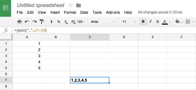
Using the JOIN function is most appropriate when linking multiple values. You only need to specify the character you want to add between the values ​​and the cell values ​​you want.

For example:

= JOIN (",", A1: A5)

We have:

1,2,3,4,5

6 useful functions in Google Sheets you may not know yet Picture 2

2. INDEX: Retrieve initial value or last value

With fixed data, spreadsheets are easy to operate. However, when adding new data regularly, such as each week adding new data streams, will require continuous editing to maintain the operation of the functions in the table.

For example, imagine you always have to calculate the change between the last cell in the table with the value ahead. And it's hard to get the results calculated in the same box at each change. Using LAST functions seems to be very appropriate, but not. The INDEX function is the solution we need. Because it allows you to retrieve the value of a cell by specifying the column and row position in the conditional array.

= INDEX (A: A, 1,1)

6 useful functions in Google Sheets you may not know yet Picture 3

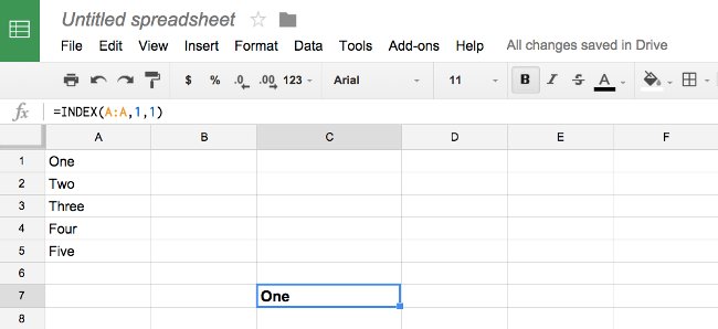
Combining INDEX with COUNTA you can create a calculation to retrieve the last value of a column.

= INDEX (A: A, COUNTA (A: A), 1)

6 useful functions in Google Sheets you may not know yet Picture 4

3. Insert data into Google Sheets

One of the great features of Google Sheets is the import function. This function allows dragging data from different sources such as XML, HTML, RSS - CSV into your spreadsheet accordingly to enter how lists of blog posts, inventory or other data from other services . For example, you can import multiple links from the URL as follows:

= IMPORTXML ("https://en.wikipedia.org/wiki/Moon_landing", "// a / @ href")

6 useful functions in Google Sheets you may not know yet Picture 5

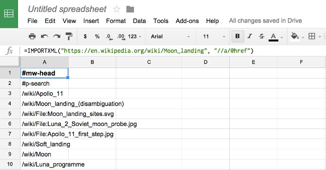
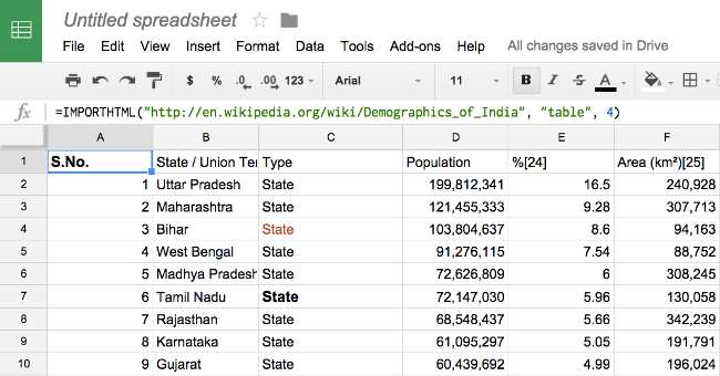
Enter the list or table content from the specified URL:

= IMPORTHTML ("http://en.wikipedia.org/wiki/Demographics_of_India", "table", 4)

6 useful functions in Google Sheets you may not know yet Picture 6

Enter RSS or Atom:

= IMPORTFEED ("http://news.google.com/?output=atom")

6 useful functions in Google Sheets you may not know yet Picture 7

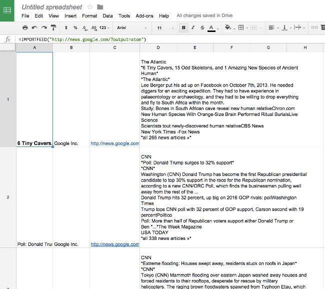
Enter the contents of the CSV file:

= IMPORTDATA ("http://www.census.gov/2010census/csv/pop_change.csv")

6 useful functions in Google Sheets you may not know yet Picture 8

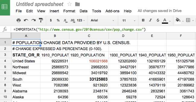
The mix of text and automatic features of Google Sheet, data entry functions have become powerful tools for screening and setting up data from public sources.

4. Vlook up and Hlookup

The following example demonstrates that Google Sheet search functions are the best. They allow searching to string a word and then read the value to the equivalent column or line. This is really useful if you have different data sets with the same object in the spreadsheet. For example, lines of data about products, personnel or projects.

In the example below, imagine you want to track the change in the number of apples, oranges, pears in January and February. The order of the available fruits varies from month to month so do not use calculations except for cells.

Instead, VLOOKUP searches the data table vertically until it finds the common point of the word and then reads in a horizontal row to find the corresponding value in the adjacent column. VLOOKUP stands for Vertical Lookup because it finds vertical and later words in a horizontal row to produce the value while Hlook the Horizontal Lookup abbreviation because it finds words in horizontal rows and then gives vertical values. .

First, with Vlookup use the following table and calculations:

= VLOOKUP (F2, $ A $ 2: $ B $ 6.2, false)

In which, "F2" the value to search for "Apple" in cell F2. Because of using Vlookup, the calculation of "$ A $ 2: $ B $ 6" of the calculation only tells Google Sheet to search along the January data sheet. "2" indicates to find "Apple" in the second column. "False" is assumed if no equivalent value is found, then they will be ignored in another location. Finally, complete the Apple search calculation in the January data table and trace the value 1003 in the second column.

To calculate the change, we need to get the search function of February minus the search function of January so there is a calculation like this:

= VLOOKUP (F2, $ C $ 2: $ D $ 6.2, false) -VLOOKUP (F2, $ A $ 2: $ B $ 6.2, false)

The second search calculation is similar to the calculation above, but now we enter the February data and get them except January data. Therefore, writing a February data search operation similar to that of January only changes "$ A $ 2: $ B $ 6" for "$ C $ 2: $ D $ 6" . Now they will take the number of apples of February (785) from the number of January (785) and retrieve the value of -218.

6 useful functions in Google Sheets you may not know yet Picture 9

Similarly, Hlookup represents the equivalent function but reads in a horizontal line and looks vertically.

5. COUNTIF and SUMIF in Google Sheets

SUMIF and COUNTIF are easier than a search function. If the logical clause in CountIF or SumIF is correct, Google Sheets can count the number of instances or sum the equivalent value.

See the example below, you can count the number of apples sold with the following calculation:

= COUNTIF (B2: B10, "Apple")

It shows that: Count the number of fields from Apple in cell B2 to B10.

6 useful functions in Google Sheets you may not know yet Picture 10

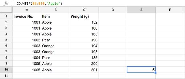
You can calculate the total weight of apples sold using SumIF function.

= SUMIF (B2: B10, "Apple", C2: C10)

It searches for the number of words Apple entered in column B and then calculates the total values ​​of the equivalent cell in column C.

6 useful functions in Google Sheets you may not know yet Picture 11

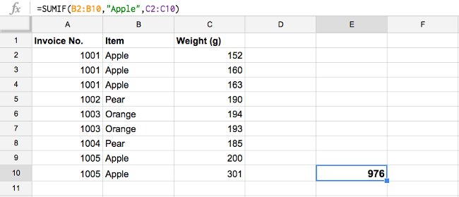
6. Table Pivot

Pivot Table is the last useful function I want to mention in this article. You can open the Pivot panel by selecting the data you want to use then clicking Data> Pivot Table .

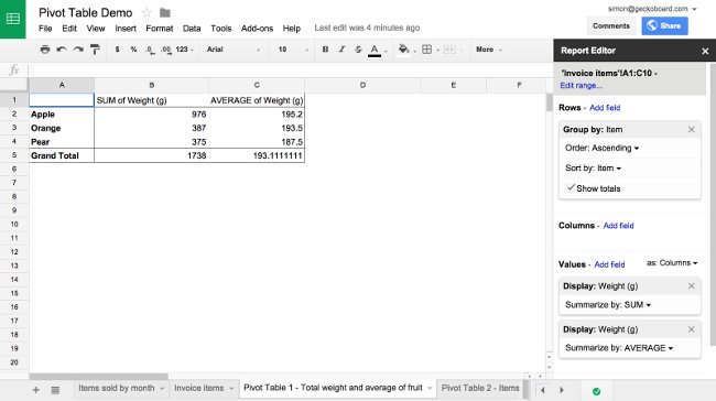
Report Pivot makes it easy to enter, filter, classify and aggregate data through the user interface. For example, with a Pivot table you will get the same results as CountIF and SumIF for all fruits without using any calculations. In addition to counting and synthesizing, it can calculate other values ​​such as average, variance as shown below.

6 useful functions in Google Sheets you may not know yet Picture 12

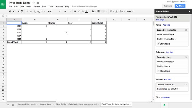
You can use Pivot tables to reconstruct data. Looking at the image below, the invoice number in the first column with each column is a type of fruit. Then, each cell indicates the number of each type in order.

6 useful functions in Google Sheets you may not know yet Picture 13