8 useful functions in Google Sheets you may not know

Google Sheets is an extremely flexible and outstanding tool that combines setting up and calculating data in spreadsheet form. It's cloud-based, so it offers lots of interactive functionality, automated data collection, and even pulls data from third-party APIs.

If you often work with spreadsheets like Excel, iWork Numbers, Zoho Sheet or Open Office Calc, you will easily use Google Sheets. If you are just starting to get acquainted with Sheets, or are learning about the Spreadsheet program, below are 8 useful functions for your data.

For more Google SpreadSheets tips click here.

1. COUNTIF and SUMIF in Google Sheets

SUMIF and COUNTIF are a bit easier than the search function. If the logical statement in CountIF or SumIF is true, Google Sheets can count the number of cases or sum the equivalent value.

Looking at the example below, you can count the number of apples sold with the following calculation:

=COUNTIF(B2:B10,"Apple")

It shows that: Count the number of fields with the word Apple in cells B2 to B10.

8 useful functions in Google Sheets you may not know Picture 1

You can calculate the total weight of apples sold using the SumIF function.

=SUMIF(B2:B10,"Apple",C2:C10)

It searches for the number from Apple entered in column B then calculates the equivalent cell sum values ​​in column C.

8 useful functions in Google Sheets you may not know Picture 2

2. VLOOKUP and HLOOKUP

The following example will prove that Google Sheets' search functions are the best. They allow searching to the string of a word and then reading the value into the equivalent column or row. This is really useful if you have different datasets with the same objects in the spreadsheet. For example, rows of data about products, personnel or projects.

In the example below, imagine you want to track the change in the number of apples, oranges, and pears in January and February. The order of available fruit varies from month to month so do not use subtraction for the cells.

Instead, the VLOOKUP function searches the table of data vertically until it finds what the words have in common and then reads horizontally to find the corresponding value in the adjacent column. VLOOKUP stands for Vertical Lookup because it looks for words vertically and then horizontally to give the value while Hlook up stands for Horizontal Lookup because it finds words horizontally and then gives the value vertically .

First, with VLOOKUP use the following table and calculations:

=VLOOKUP(F2,$A$2:$B$6,2,false)

In which, "F2" is the search value of "Apple" in cell F2. Because we use VLOOKUP, the "$A$2:$B$6" of the calculation tells Google Sheet to search along the January data table. "2" indicates searching for "Apple" in the second column. "False" is the assumption that if no equivalent value is found, we will skip it and search in another location. Finally, complete the calculation looking for Apple in the January data table and find the value 1003 in the second column.

To calculate the change, we need to subtract January's search function from February's search function, so the calculation is as follows:

=VLOOKUP(F2,$C$2:$D$6,2,false)-VLOOKUP(F2,$A$2:$B$6,2,false)

The second search calculation is similar to the one above, but now we import the February data and subtract the January data from them. So, write the same search calculation for February's data as for January's just substituting "$A$2:$B$6" for "$C$2:$D$6" . Now we will subtract February's quantity of apples (785) from January's quantity (785) and get the value -218.

8 useful functions in Google Sheets you may not know Picture 3

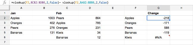
Similarly, HLOOKUP represents the equivalent function but reads horizontally and looks vertically.

3. IMPORTRANGE

IMPORTRANGE is a useful function if you need to get data from different Google Sheets worksheets. Instead of copying data from one worksheet and pasting it into another desired worksheet, you can use this formula to save time.

If someone other than you owns the worksheet, you must have access to the worksheet before you can start using the IMPORTRANGE function.

During the process of pulling data from different worksheets, any data changes on the source sheet will automatically reflect on the target sheet.

Therefore, this is an essential formula if you are creating reports or dashboards by sourcing data from different members of your project team.

In the video above, you can see how to easily import US demographic data from one worksheet to another. You just need to mention the sheet URL, sheet name, and the data range you want to import.

This formula does not import any visual formatting from the source. You can use the following formula syntax if you want to try it out:

=IMPORTRANGE("URL","Sheet1!B3:R11")

4. IFERROR

Your spreadsheet can get messy if there are too many errors. The error often occurs when you apply multiple formulas across columns and sheets, but don't have much data to return any values.

If you share such files with team members or customers, they may not be pleased. Furthermore, it will be difficult for you to avoid making mistakes when completing the work. The IFERROR function will come to your rescue.

Place your formula inside the IFERROR function and mention what text to display if there is an error. The video above shows the use of IFERROR in situations when you manage spreadsheets for product pricing or student classification.

Here's the formula syntax that might be useful if you want to try it yourself:

=iferror(D4/C4, 0) =iferror(VLOOKUP(A23,$A$13:$G$18,7,false),"ID Mismatch")

5. ARRAYFORMULA

This function helps you reduce the time you spend editing formulas in your spreadsheet. When you need to apply functions to thousands of rows and columns in a worksheet, you should use ARRAYFORMULA instead of non-array functions.

Non-array functions are functions that you create in one cell and then copy-paste them into another cell in the worksheet. The Google Sheets program is smart enough to modify formulas according to cell addresses. However, by doing so, you will open up the following problems:

1. The worksheet becomes slow because of the individual functions in thousands of cells.
2. Making any changes to the formula will require hours of editing.
3. Copying and pasting non-array formulas into specified cells is a tiring process.

Let's say that you are responsible for creating a spreadsheet document with student names, grades by subject, and the student's total score. Now, if you have to calculate scores for not just a few students in a class, but all students across the city, a formula based on the regular `+` operator will be time-consuming. You can use ARRAYFORMULA as mentioned below.

=ArrayFormula(B2:B+C2:C+D2:D+E2:E+F2:F)

In this formula, the range B2:B specifies infinite. You can make it finite by editing the range to B2:B10 , etc.

6. FILTER

While you can easily filter and sort your data by going to Data > Create a Filter , it's easier to just use the FILTER function to get the results you want to see. The parameters are very simple:

=FILTER(phạm vi, điều kiện1, điều kiện khác)

The 'other conditions' section is optional. These are essentially true/false comparisons of other cells to further filter your results.

1. In an empty cell, start your formula. Ideally you would create the same column headings as the data you are filtering, then start the formula in the first cell below your first column heading. For example, the article is filtering for employee IDs with salaries greater than $120,000.

8 useful functions in Google Sheets you may not know Picture 4

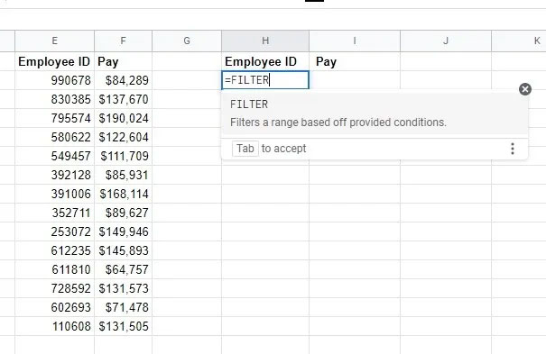
2. Enter your range and first condition. You can close the formula here or enter additional conditions separated by commas. In the example, the condition is to select only values ​​in the range F2:F14 above $120,000.

8 useful functions in Google Sheets you may not know Picture 5

3. Your results will appear under the new column header (if you have one).

8 useful functions in Google Sheets you may not know Picture 6

The great thing about this formula is that if you make any changes to your data, the results will automatically update. Add a new row in the original range and it will be included automatically. This is a much more dynamic option than the filters in the Google Sheets menu.

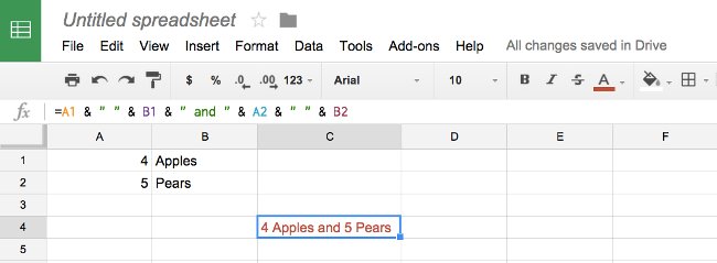
7. JOIN

The JOIN function is used to deepen a string of values ​​into a text for convenience of use. Or simply synthesize a few key values ​​or some HTML.

Type & to connect the values ​​of different cells, and use quotation marks with whatever text you want to insert.

For example, we use the following calculation:

=A1 & " " & B1 & " and " & A2 & " " & B2

and the result is "4 Apples and 5 Pears"

8 useful functions in Google Sheets you may not know Picture 7

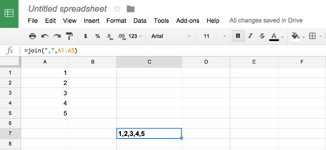
Using the JOIN function is most appropriate when joining multiple values. You just need to indicate the character you want to add between the values ​​and the cell values ​​you want.

For example:

=JOIN(",",A1:A5)

We have:

1,2,3,4,5

8 useful functions in Google Sheets you may not know Picture 8

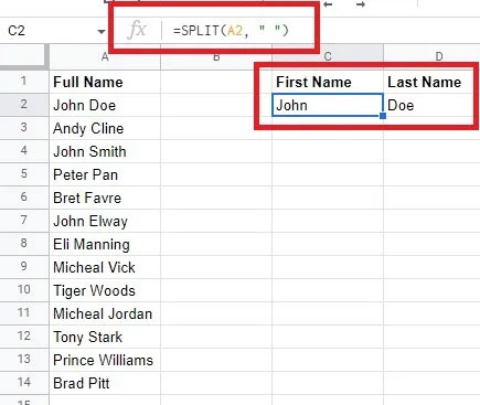
8. SPLIT

Do you have the opposite problem and need to separate items within a cell? Just use the SPLIT function. It is the opposite of the JOIN function. For example, you may want to separate first names and last names to make it easier to sort data alphabetically by last name.

For SPLIT, the parameters are:

SPLIT(văn_bản, dấu_phân_tách, [tách_theo_mỗi], [xóa_văn_bản_trống])

More simply, 'text' is the cell you want to split, separator is the character used to specify where to split the text, and the last two parameters are optional. split_by_each  refers to the fact that you want to split at every matching character. delete_blank_text removes blank text from your results. It is set to TRUE by default.

You will need two or more blank cells, one for each section of text that will be divided. The example is splitting the full name into first and last names, so only two blank cells are needed.

1. In your first blank cell, start your formula with =SPLIT(

2. Enter the cell you want to split.

3. Enter the separator you want. In this example, it's a space, so " " will be used, but this could be anything, such as a letter or symbol.

4. Close your formula and fill multiple cells in the same row.

8 useful functions in Google Sheets you may not know Picture 9

You can apply the above Google Sheets functions in many different cases. Surely you can find many new situations to apply these formulas. They will save time and help you interpret data in an easy-to-understand way.

Jessica Tanner

Update 15 July 2024