6 Conditional Functions That Make Excel Spreadsheets Smarter

Many people use Excel for basic spreadsheets, but you need to do more than just calculate simple calculations. If your formulas get complicated, conditional functions are a smarter option, hiding in plain sight. They handle complex logic and automate decisions without requiring you to go through a steep learning curve.

 

6. IF and IFS Functions: Handling Simple and Complex Decisions

The IF function is Excel's most basic decision-making tool. It evaluates a condition and returns one value if the condition is true, another value if the condition is false—kind of like Excel asking "what if?" and responding accordingly.

Here's a real-world example. Let's say you're managing employee performance data and need to automatically categorize ratings. Anyone with a score above 3.5 would be marked as "Satisfactory," while everyone else would be marked as "Needs Improvement." You could use an IF function as shown in the following formula to do this across hundreds of employees.

=IF(C2>3.5, "Satisfactory", "Needs Improvement")

But what about the case of multiple results, as traditional nested IF statements can become extremely difficult, as illustrated below.

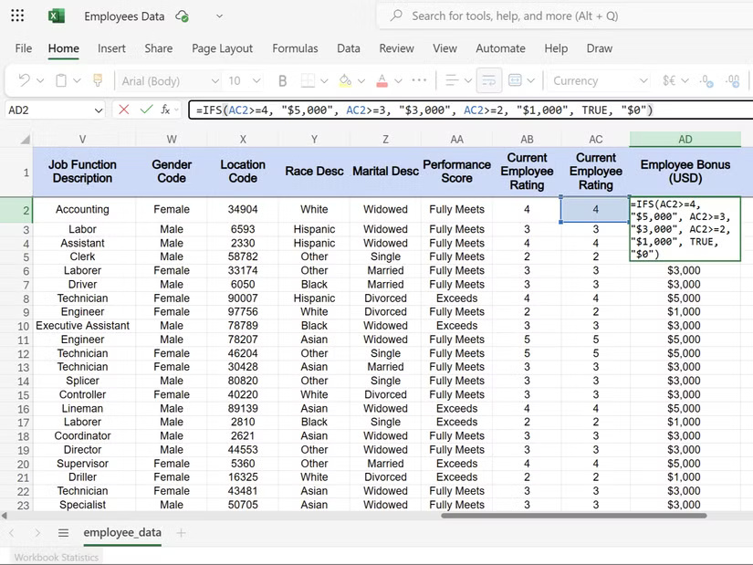
=IF(C2>=4.5, "Excellent", IF(C2>=3.5, "Good", IF(C2>=2.5, "Average", "Poor")))

That's where IFS comes in handy. The IFS function effectively manages many situations. To calculate employee bonuses based on performance levels, you can use the IFS function as shown in the following formula.

=IFS(AC2>=4, "$5,000", AC2>=3, "$3,000", AC2>=2, "$1,000", TRUE, "$0")

 

5. SWITCH function: Simplify value matching

The SWITCH function is a better choice when you need to match an exact value, because it doesn't involve greater than or less than logic; instead, it involves a direct lookup. Each value-result pair acts like a dictionary entry, which makes its syntax simple.

=SWITCH(lookup_value, value1, result1, value2, result2, default_result)

Consider the employee department code in the HR spreadsheet. If you use the IF function, the formula becomes long and complicated, as shown in the following example.

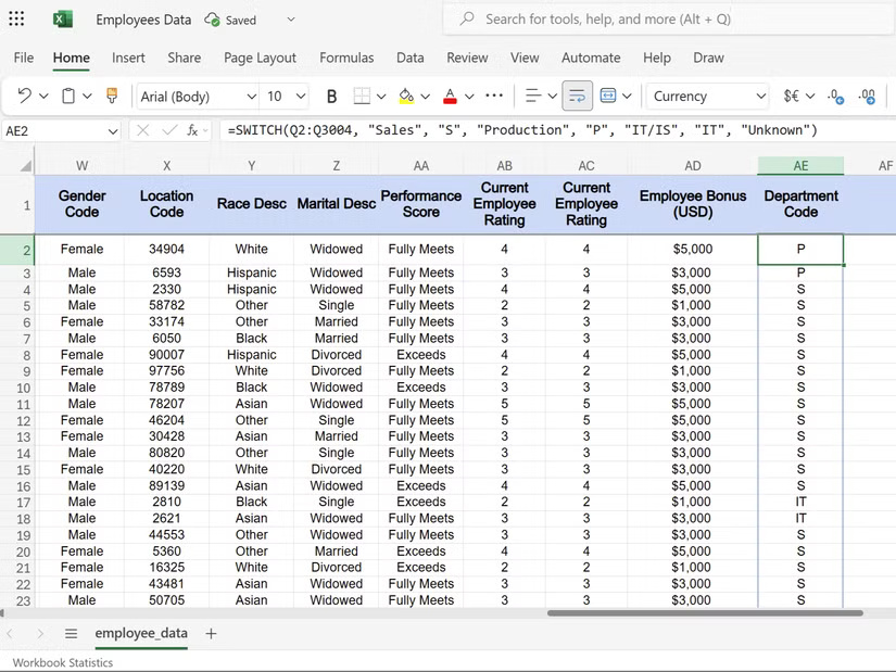
=IF(B2="HR", "Human Resources", IF(B2="IT", "Information Technology", IF(B2="FIN", "Finance", "Unknown")))

Instead, you can use SWITCH for more efficient handling.

=SWITCH(Q2:Q3004, "Sales", "S", "Production", "P", "IT/IS", "IT", "Unknown")

 

4. CHOOSE function: Select value by position

The CHOOSE function works like a numbered list; you provide a position number, and it returns the corresponding value from the predefined options. This is Excel's way of saying, "Give me item number 3 in this list."

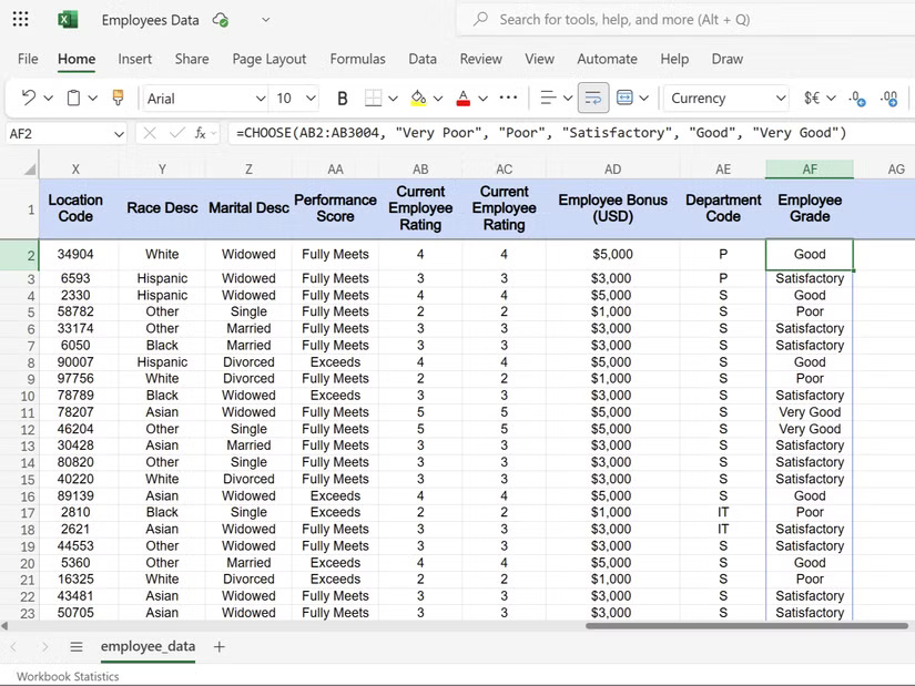
The syntax is simple. The first argument is the position number, followed by your list of values. Continuing with the employee spreadsheet example, you can use this function to convert the scores into a readable description:

=CHOOSE(AB2:AB3004, "Very Poor", "Poor", "Satisfactory", "Good", "Very Good")

This formula takes the numbers in column AB and returns the employee's corresponding score. Position one results in "Very Poor", position two results in "Poor", etc.

The CHOOSE function is especially useful for quarterly reports. You can convert quarter numbers into labels that are suitable for charts and presentations:

=CHOOSE(E2, "Q1 2024", "Q2 2024", "Q3 2024", "Q4 2024")

3. AND and OR Functions: Building Complex Logic

The AND and OR functions handle multiple-condition situations that cannot be handled by a single IF statement. AND requires that each condition be true. For example, an employee's promotion requirements might require consideration of both 2 years of service and a performance rating of 3.5 or higher, as shown in the following formula.

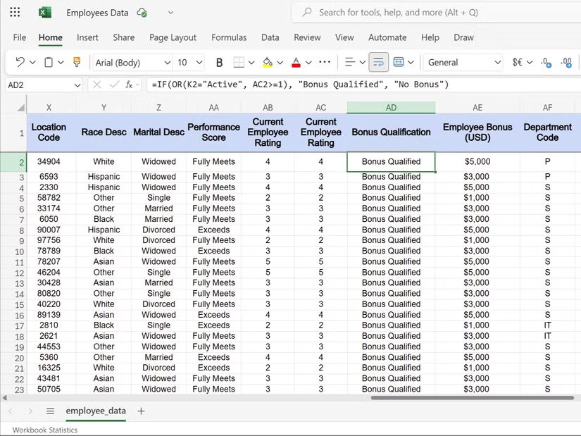
=IF(AND(C2>2, D2>3.5), "Eligible", "Not Eligible")

But OR takes the opposite approach – it only requires one condition to be true. Let's say you have to check for bonus eligibility; only active employees can qualify if they have good performance:

=IF(OR(K2="Active", AC2>=1), "Bonus Qualified", "No Bonus")

 

2. SUMIFS, COUNTIFS and AVERAGEIFS functions: Analyzing data with conditions

These three functions transform raw data into useful insights by applying multiple conditions simultaneously. They can be used to analyze large data sets without the need for pivot tables.

For example, an HR person might want to analyze total salaries for specific departments, the number of employees for certain job levels, or average performance ratings by group. These functions handle such multi-criteria analysis with ease.

The SUMIFS function adds values that meet multiple criteria. When calculating the total salary for IT employees with more than 3 years of experience, the formula becomes:

=SUMIFS(E:E, B:B, "IT", D:D, ">3")

The syntax follows a logical pattern: Sum range, criteria range 1, criteria 1, criteria range 2, criteria 2. You can add up to 127 pairs of conditions for specific calculations.

On the other hand, the COUNTIFS function counts cells that meet multiple conditions. To determine the number of marketing employees with a performance rating above 4.0, we will use the following formula.

=COUNTIFS(B:B, "Marketing", F:F, ">4")

This formula identifies high performers by department, helping to identify potential candidates for promotion or training needs across the organization.

The AVERAGEIFS function calculates an average based on multiple criteria. To find the average salary of senior executives in the finance industry, we would use:

=AVERAGEIFS(E:E, B:B, "Finance", C:C, "Senior")

The above formula calculates the average salary of senior employees in the Finance department.

1. IFERROR and IFNA Functions: Preventing Annoying Error Messages

Nothing ruins a professional spreadsheet like #DIV/0! or #N/A errors scattered throughout your data. The IFERROR and IFNA functions help you troubleshoot common Excel errors and replace annoying error messages with more meaningful alternatives.

The IFERROR function catches errors and replaces the value you select. For example, when calculating employee performance ratings, dividing by zero will produce an error. Instead of displaying #DIV/0! , you can choose to display more useful information:

=IFERROR(C2/D2, "No Data Available")

This formula attempts division but will display "No Data Available" if an error occurs, which is a more concise way of saying it.

On the other hand, the IFNA function specifically targets the #N/A error from lookup functions. When we look up information using the VLOOKUP function, missing data will generate the #N/A error . To avoid this, we can use the IFNA function as in the following formula.

=IFNA(VLOOKUP(A2, A2:AG3004, 4, FALSE), "Employee Not Found")

This formula looks up the employee ID in column A2 within your employee list and returns the name from the fourth column. When the employee ID does not exist in your database, instead of displaying the #N/A error, it displays the user-friendly message "Employee Not Found".

The main difference is that the IFERROR function catches everything, such as division errors, reference errors, and lookup errors. IFNA only handles #N/A errors, allowing other types of errors to display normally.