How to Create the Idea of an Idea Image

The Tutorial

1. How to Create the Idea of an Idea Image Picture 1
   How to Create the Idea of an Idea Image Picture 2
   Open a new Excel workbook and create 5 worksheets named: Data, Goal Looker, Rose, Chart and Saves unless working from the workbook formerly created, Create a Cyclical Chart Using Spheroids or Create a Dakini and Boddhisattva Aspect of the Mother Planet. If using one of those workbooks saved under a new name for this article, look for the word NEW or MODIFIED by the Step or Sub-Step (as otherwise all but the last few steps on creating the unique chart were directly copied and organized into sub-steps were directly copied from Create a Dakini and Boddhisattva Aspect of the Mother Planet). Save the workbook under the filename that makes sense to you in your line of endeavor. The source file for these articles is "Eggies.xlsx". It is presumed you've copied and renamed "How to Create a Dakini and Boddhisattva Aspect of the Mother Planet" as far as the NEW and MODIFIED and MODIFIED AGAIN comments apply.
2. Open Preferences. Recommended Settings: Set General to R1C1 Off and Show the 10 Most Recent Documents; Edit - set all the Top options to checked except Automatically Convert Date System. Display number of decimal places = blank (for integers preferred), Preserve display of dates and set 30 for 21st century cutoff; View - show Formula Bar and status bar, hover for comments and all of Objects, Show gridlines and all boxes below that auto or checked; Chart - show chart names and data markers on hover. Leave rest unchecked for now; Calculation -- Automatically and calculate before save, max change .000,000,000,000,01 w/o commas if you do goal-seeking a lot and save external link values and use 1904 system; Error checking - check all; Save - save preview picture with new files and Save Autorecover after 5 minutes; Ribbon -- all checked except Hide group titles and Developer.
3. Create Defined Name variables:

   1. In the cell range A1:N1, input the following Variable Names: A1: AjRows; B1: GM (for Golden Mean); C1: Factor1; D1: Factor2; E1: Number; F1: NewDate1; G1: GMSL (for Golden Mean Short Leg); H1: KEY; I1: KEY2_; J1: Variable; M1 Eggies4; N1: ShrinkExpand4
   2. Select cell range A1:N2 and Insert Name Create (Create Names in) Top Row. Select cell range A2:N2 and do Format Cell Border Outline Center Vertical Center Horizontal Black Bold. Do Format Cell Font Color (fire engine) Red. That is because typically these variables won't be changed.
   3. In the cell range A3:L3, input the following Variable Names: A3: Tip B3: Base; C3: Spheroids; D3: ShrinkExpand; E3: PiDivisor F3: NewDate2; G3: Base2; H3: Spheroids2; I3: ShrinkExpand2; K3: ShrinkExpand3; L3: Base4
   4. Select cell range A3:L4 and Insert Name Create (Create Names in) Top Row. Select cell range A4:L4 and do Format Cell Border Outline Center Vertical Center Horizontal Black Bold.. Do Format Cell Font Color (fire engine) Red. That is because typically some of these variables will change but most will not.
   5. Input variable values in row 2: A2: input 2880; Insert New Comment and edit in 2880.
   6. B2: input "=(-(1-SQRT(5))/2)^IF(Spheroids<24,1,1)" and Insert New Comment and edit in "Original formula =(-(1-SQRT(5))/2)^IF(Spheroids<24,1,1)"
   7. C2: input "=VLOOKUP(ABS(Spheroids),LOOKER,IF(Spheroids<=24,2,3))" and Insert New Comment and edit in "Original formula =VLOOKUP(ABS(Spheroids),LOOKER,IF(Spheroids<=24,2,3))"
   8. D2: Input "=VLOOKUP(ABS(Spheroids),LOOKER,IF(Spheroids<=24,2,2))" and Insert New Comment and edit in "Original formula =VLOOKUP(ABS(Spheroids),LOOKER,IF(Spheroids<=24,2,2))"
   9. E2: Input 1. This variable, Number, is not being used at present. It's purpose is to warp or skew the output via incorporation into the formulas in cell range C6I2886. Insert a New Comment if you like.
   10. F2: Input "=1954/9/2". This variable, NewDate1, is not being used at present. It's purpose is to warp or skew the output personally via incorporation into the formulas in cell range C6:I2886. It is a birth date in format yyyy/mm/dd, i.e. a double quotient. Insert a New Comment if you like.
   11. G2: Input "=1-(-(1-SQRT(5))/2)^IF(Spheroids<24,1,1)" and Insert New Comment and edit in "Original formula =1-(-(1-SQRT(5))/2)^IF(Spheroids<24,1,1)".
   12. H2: Input "=IF(Spheroids>=30,Spheroids/30,Spheroids)" w/o the quotes. Insert New Comment and edit in "Keeps Spheroids round. Formula now is =IF(Spheroids>=30,Spheroids/30,Spheroids)". Expand the comment frame if need be.
   13. MODIFIED AGAIN: I2: Input "=IF(Spheroids>=30,Spheroids,Spheroids2)*0.5" w/o the quotes. Insert New Comment and edit in "Keeps Spheroids2 round. New formula is =IF(Spheroids>=30,Spheroids,Spheroids2)*0.5 Old formula did not multiply by .5". Expand the comment frame if need be.
   14. In J2, enter 1.
   15. In M2, enter 100.
   16. In N2, enter .1
4. Select cell R8 and enter LOOKER2 for the entry of that table.

   1. Edit Go To cell range R9:R108 and with R9 the active high-lighted cell, do Edit Fill Series Columns Linear Step Value 1 OK.
   2. Enter .01 into cell S9; enter .35 into cell S14; enter .5 into cell S20; enter .75 into cell S26; and enter 1 into cell S32. Do Edit Fill Series Columns Linear Accept proposed Step Value OK for each sub-range just entered above, i.e. from .01 to .35, from .35 to .5, from ,5 to .75, and from .75 to 1.
   3. Edit Go To cell range S32:S108 and with S32 the active high-lighted cell, do Edit Fill Series Columns Linear Step Value .04166667
   4. Edit Go To cell range R9:S108 and Insert Name Define LOOKER2 to cell range $R$9:$S$108. Format Cells Border fire engine Red Bold Outline.
   5. Note that .125*240- = 30 Spheroids. 1/24 = 1/8 * 1/3 = .0416667 and 240/2880 = 1/12th. Or, another way of saying it is that 2880/30 = 96 spiralling data points per spheroid. This is what is meant when it is said the formula achieves good roundness, i.e. is a good sphere.
5. Save the workbook.
6. Input variable values in row 4:

   1. A4: input "=Base*12/(VARIABLE/1)*PI()"; Insert New Comment and edit in "Original formula =Base*12/(VARIABLE/1)*PI()". Expand the comment frame if need be.
   2. B4: Input "=16*107". Insert New Comment and edit in "Original constant value =16*107."
   3. C4: Input 100. Do Insert New Comment and edit in comment "See Lookup Tables for range of Spheroids values contemplated by this worksheet. Now=100." Expand the comment frame if need be.
   4. MODIFIED: D4: Input 1.1 and do Insert New Comment and edit in comment "Input 1 if keeping input data for Spheroids normalized, else 2 to shrink by 1/2, or .5 to expand by a factor of 2, since ShrinkExpand is a Divisor. Now =1.1" Expand the comment frame if need be.
   5. E4: Input 180. Do Insert New Comment and edit in comment "Normally this will not be changed from 180, but can be for warping effects. Original value 180". Expand the comment frame if need be.
   6. F4: Input "=(1958/4/13)". This variable, NewDate2, is not being used at present. It's purpose is to warp or skew the output personally via incorporation into the formulas in cell range C6: I2886. It is a birth date in format yyyy/mm/dd, i.e. a double quotient. Insert a New Comment if you like.
   7. G4: Input "=16*107". Insert New Comment and edit in "Original constant value =16*107."
   8. H4: Input 12. Insert New Comment and edit in "=Spheroids is original formula because most often Spheroids2 is the Standard or Goal for Spheroids, and needs to correspond per period on a 1:1 basis. Was 40. Now =12." Expand the comment frame if need be.
   9. I4: Input "=(1/E2890)^(3/2)". Insert New Comment and edit in "Original formula =ShrinkExpand is most usual value as Standard or Goal, e.g. 100% of Normal. But if 80% of Normal is the New Goal, say for a Personal Fitness Program, then a little math is required.  ShrinkExpand2 = 1/.80, or 1.25 would be the new input. This is because it was thought the natural trend would be to want to shrink by say a factor of 2, so 2 = 1/.50 and the New Goal is to be 50% of Normal, or shrink by a factor of 2 (as a divisor). You may change the formulas and comments so that ShrinkExpand and ShrinkExpand2 are multiplicative instead of divisive if preferred. Was 1.19122798149309. Now =(1/E2890)^(3/2)" Expand the comment frame if need be. In cell E2890 should be the formula "=MAX(E6:E2886)"and above it the MIN formula.
   10. MODIFIED AGAIN: K4: Input 0.014 and Insert New Comment with this value as what's now current.
   11. L4: Input "=16*107"
7. MODIFIED: Input the Column Headings across row 5. A5: Base t; B5: c; C5: Cos; D5: Sin; E5: Main X; F5: Main Y; G5: Count2; H5: Second X; I5: Second Y; J5: Rose X; K5: Rose Y; L5: Count4; M5: EGGIES X; N5: EGGIES Y. Select cell range A5:I5 and Format Cell Font Underline. Select the following cells with Shift+Command: C4, D4, F4. G4, H4, I4, K4, L4, C2, D2, E2, F2, H2, I2, J2, M2, N2 and Format Cell Fill canary yellow (for input cells) and Font size 14. Format Cells A4:L4 Number Number Decimal Places 4 and select column range A:N and do Format Column Autofit Selection.
8. Save the workbook.
9. Enter the columnar formulas:

   1. Cell A6: Input "=IF(ODD(Spheroids)=Spheroids,0,Tip)" and do Insert Comment and edit comment "Original formula =IF(ODD(Spheroids)=Spheroids,0,Tip)". Expand the comment frame if need be. Do Format Cell Fill Light Rose color to distinguish it from the other cells in the column.
   2. Edit Go To cell range A7:A2886 and with A7 the active high-lighted cell, input "=(A6+(-Tip*2)/(AjRows))" and do Edit Fill Down. Select cell A7 and copy the the formula in the formula bar and do Insert New Comment and edit comment "Original formula "=(A6+(-Tip*2)/(AjRows)) to bottom A2886 (as adjusts per cell on the way down)". Expand the comment frame if need be.
   3. Cell B6: Input "=IF(Spheroids<=24,Base*24/Spheroids,Base*24/Spheroids)" and do In sert New Comment and edit in "Original formula "=IF(Spheroids<=24,Base*24/Spheroids,Base*24/Spheroids)".
   4. Edit Go To cell range B7:B2886 and with B7 the active high-lighted cell, input "=B6" and do Edit Fill Down. Select cell B7 and copy the the formula in the formula bar and do Insert New Comment and edit comment "Original formula =B6 to bottom B2886 (as adjusts per cell on the way down)". Expand the comment frame if need be.
   5. Edit Go To cell range C6:C2886 and with C6 the active high-lighted cell input "=Spheroids/KEY*(COS((ROW()-6)*Number*PI()/PiDivisor*Factor1))" and do Edit Fill Down. Select cell C6 and do Insert New Comment and edit it "Original Formula =Spheroids/KEY*(COS((ROW()-6)*Number*PI()/PiDivisor*Factor1))". Expand the comment frame if need be. This formula and the next one form the ring the Spheroids occupy, By taking the cosine of the cell 6 rows above the cell it's in, C6, the formula is taking the cosine of 0, which = 1.
   6. Edit Go To cell range D6:D2886 and with D6 the active high-lighted cell input "=Spheroids/KEY*(SIN((ROW()-6)*Number*PI()/PiDivisor*Factor1))" and do Edit Fill Down. Select cell D6 and do Insert New Comment and edit it "Original Formula =Spheroids/KEY*(SIN((ROW()-6)*Number*PI()/PiDivisor*Factor1)). By taking the sine of the cell 6 rows above the cell we're in, C6, the formula is taking the sine of 0, which = 0. Therefore, between the formula in C6 and the one in D6, the {x,y} coordinates of the first cell would be {1,0} if nothing else were affecting them. It proceeds counterclockwise from there. so that is how to read the chart, from 0 degrees counter clockwise back to 360 degrees. Even though there are basically 2880 rows being charted, and 2880/360 = 8, Factor1 = 1/8th at .125, so a level of detail is achieved while keeping everything normalized for a single cycle in the typical case.
   7. Edit Go To cell range E6:E2886 and with E6 the active high-lighted cell, input the formula, "=((SIN(A6/(B6*2))*GM*COS(A6)*GM*(COS(A6/(B6*2)))*GM)+C6)*VLOOKUP(ROW(),SpreadLooker,3)/ShrinkExpand" w/o quote marks and do Edit Fill Down. Select cell E6 and do Insert New Comment "Original Formula =((SIN(A6/(B6*2))*GM*COS(A6)*GM*(COS(A6/(B6*2)))*GM)+C6)*VLOOKUP(ROW(),SpreadLooker,3)/ShrinkExpand multiplies each term of the standard formula for a spherical helix per 'CRC Standard Curves and Surfaces' by David von Seggern, 1993, by GM (Golden Mean) to keep things proportional, with the z dimension added into the x and y dimensions. This is then multiplied by the Lookup Table SpreadLooker, which either randomizes the data or accepts inputs per the Goal Looker worksheet. Lastly, it is subject to ShrinkExpand, a variable for normalizing or growing or shrinking its chart relative to the Standard or Goal chart data series of Second X and Second Y." Expand the comment frame as much as necessary. I realize that there may be #NAME? error values -- these will be fixed in a little while when the Lookup Tables are completed.
   8. Edit Go To cell range F6:F2886 and with F6 the active high-lighted cell, input the formula,"=((SIN(A6/(B6*2))*GM*SIN(A6)*GM*(COS(A6/(B6*2)))*GM)+D6)*VLOOKUP(ROW(),SpreadLooker,3)/ShrinkExpand" w/o quote marks and do Edit Fill Down. Select cell F6 and do Insert New Comment "Original Formula =((SIN(A6/(B6*2))*GM*SIN(A6)*GM*(COS(A6/(B6*2)))*GM)+D6)*VLOOKUP(ROW(),SpreadLooker,3)/ShrinkExpand (see note in E6 for details)." I realize that there may be #NAME? error values -- these will be fixed in a little while when the Lookup Tables are completed.
   9. Cell G6: Input "=IF(Spheroids2<=24,Base2*24/Spheroids2,Base2*24/Spheroids2)" and do Insert New Comment and edit in "Original formula =IF(Spheroids2<=24,Base2*24/Spheroids2,Base2*24/Spheroids2)".
   10. Edit Go To cell range G7:G2886 and with G7 the active high-lighted cell, input the formula,"=G6". Do Insert New comment and edit in "Original Formula =G6 down to G2886 as adjusts per cell thereto."
   11. MODIFIED: Edit Go To cell range H6:H2886 and with H6 the active high-lighted cell, input the formula,"=((SIN(A6/(G6*2))*GM*COS(A6)*GM*(COS(A6/(G6*2)))*GM)+Spheroids2/KEY2_*(COS((ROW()-6)*Number*PI()/PiDivisor*Factor2)))/ShrinkExpand2" w/o quotes and Edit Fill Down. Do Insert Comment and edit comment "Original formula =((SIN(A6/(G6*2))*GM*COS(A6)*GM*(COS(A6/(G6*2)))*GM)+Spheroids2/KEY2_*(COS((ROW()-6)*Number*PI()/PiDivisor*Factor2)))/ShrinkExpand2 with ShrinkExpand2 being the Goal or Standard the Spheroids of Main X and Main Y are to attain."
   12. Edit Go To cell range I6:I2886 and with I6 the active high-lighted cell, input the formula,"=((SIN(A6/(G6*2))*GM*SIN(A6)*GM*(COS(A6/(G6*2)))*GM)+Spheroids2/KEY2_*(SIN((ROW()-6)*Number*PI()/PiDivisor*Factor2)))/ShrinkExpand2" w/o quotes and Edit Fill Down. Do Insert Comment and edit comment "Original formula =((SIN(A6/(G6*2))*GM*SIN(A6)*GM*(COS(A6/(G6*2)))*GM)+Spheroids2/KEY2_*(SIN((ROW()-6)*Number*PI()/PiDivisor*Factor2)))/ShrinkExpand2 with ShrinkExpand2 being the Goal or Standard the Spheroids of Main X and Main Y are to attain."
   13. Edit Go To cell range J6:J2886 and with J6 the active high-lighted cell, input the formula "=ROSE!C6/(ShrinkExpand3)" and Edit Fill Down, which may have errors if there is not a ROSE worksheet yet. Do Insert New Comment and edit in "Original formula =ROSE!C6/(ShrinkExpand3) as refers to the Rose worksheet."
   14. Edit Go To cell range K6:K2886 and with K6 the active high-lighted cell, input the formula "=ROSE!D6/(ShrinkExpand3)" and Edit Fill Down, which may have errors if there is not a ROSE worksheet yet. Do Insert New Comment and edit in "Original formula =ROSE!D6/(ShrinkExpand3) as refers to the Rose worksheet."
   15. Select cell L6 and enter the formula w/o quotes "=IF(Eggies4
   16. Edit Go To cell range L7:L2886 and with L7 active and high-lighted, enter the formula w/o quotes "=L6" and Edit Fill Down. Do Insert New Comment and edit in "Original formula =L6".
   17. Edit Go To cell range M6:M2886 and with M6 the active high-lighted cell, input the formula,"=((SIN(A6/(B6*2))*GM*COS(A6)*GM*(COS(A6/(B6*2)))*GM)+C6)*VLOOKUP(ROW(),SPREADLooker,4)/ShrinkExpand4" w/o quotes and Edit Fill Down. Do Insert Comment and edit comment "Original formula =((SIN(A6/(B6*2))*GM*COS(A6)*GM*(COS(A6/(B6*2)))*GM)+C6)*VLOOKUP(ROW(),SPREADLooker,4)/ShrinkExpand4"
   18. Edit Go To cell range N6:N2886 and with N6 the active high-lighted cell, input the formula,"=((SIN(A6/(B6*2))*GM*SIN(A6)*GM*(COS(A6/(B6*2)))*GM)+D6)*VLOOKUP(ROW(),SPREADLooker,4)/ShrinkExpand4" w/o quotes and Edit Fill Down. Do Insert Comment and edit comment "Original formula =((SIN(A6/(B6*2))*GM*SIN(A6)*GM*(COS(A6/(B6*2)))*GM)+D6)*VLOOKUP(ROW(),SPREADLooker,4)/ShrinkExpand4"
   19. NEW: Save the workbook.
10. Create the Rose worksheet with the new HOLE column J.

    1. Create a new worksheet via Insert Worksheet or the Plus button at the right end of the worksheet tabs and name it ROSE if not done already.
    2. Enter the Row 1 headings: B1: Top; C1: Changed:  G1: a; H1: n; I1: Converter; J1: Converter_Y
    3. Select cell range B1:J2 and Insert Name Create Names in Top Row.
    4. Enter the values of row 2: B2: -4; C2: Graphing D2: Graphing G2: "=SQRT(MIN('GOAL LOOKER'!B2:B65))" which will cause an error until the Goal Looker worksheet is done. H2: 45; I2: .01; J2: "=Converter"
    5. NEW: Select cell I3 and enter HOLE and align right. Select cell J3 and enter .15 and Format Cells Border Black bold Outline Fill Yellow Font red. Insert Name Define Name Hole to cell $J$3. Do Insert New Comment and edit in "Original value .15 for hole in middle of closed or open rose. X and Y now refer to this column."
    6. NEW: Select cell J5 and enter p^2 - HOLE.
    7. NEW: Edit Go To cell range J6:J2886 and enter w/o quotes and with J6 active the formula "=IF(ABS(I6)
    8. Enter the Headings in row 5. A5: Theta ø; B5: Series; C5: x; D5: y; E5: r; F5: ø; G5: a^2; H5: sin n Theta I5: p^2
    9. MODIFIED AGAIN: Select cell C4 and enter "=I4*COS(Theta*Converter)+COS((ROW()-6)*PI()/180)" as a formula reminder of how to get the rose to open with a receptacle.
    10. NEW: Select cell D4 and enter "=I4*SIN(Theta*Converter_Y)+SIN((ROW()-6)*PI()/180)" for the same reason. These will produce #VALUE! errors, which is OK for now.
    11. Edit Go To A6:A2886 and enter 0 in A6 and Edit Fill Series Columns Linear Step Value 1 OK. Insert Name Define name Theta for cell range $A$6:$A$2886.
    12. Select cell B6 and enter "=Top" and Format Cells Light Blue.
    13. Edit Go To cell range B7:B2886 and enter "=B6-Top/360" and Edit Fill Down. Do Insert New Comment and edit in "Original formula =B6-Top/360".
    14. NEW+MODIFIED AGAIN: Edit Go To cell range C6:C2886 and enter "=J6*COS(Theta*Converter)" and Edit Fill Down. Do Edit Comment and edit in "Original formula =I6*COS(Theta*Converter) was =I6*COS(Theta*Converter_Y)+COS((ROW()-6)*PI()/180) and is now =J6*COS(Theta*Converter) for closed rose with hole".
    15. NEW+MODIFIED AGAIN: Edit Go To cell range D6:D2886 and enter "=J6*SIN(Theta*Converter_Y)" and Edit Fill Down. Do Insert New Comment and edit in "Original formula =I6*COS(Theta*Converter_Y) was =I6*SIN(Theta*Converter_Y)+SIN((ROW()-6)*PI()/180)and is now =J6*SIN(Theta*Converter_Y) for closed rose with hole".
    16. Select cell C2888 and enter "=I2888*COS(Theta*Converter)" which is the closed rose formula.
    17. Select cell D2888 and enter "=I2888*SIN(Theta*Converter)" which is the closed rose formula. This will result in #VALUE! errors which are OK for now.
    18. NEW: Copy C2886:D2886 and Paste to C2890 and in E2890, aligned left note that This is closed rose with hole formula." There will be #VALUE! errors, which are acceptable for now.
    19. Edit Go To cell range E6:E2886 and enter "sqrt(I6)" and Edit Fill Down.
    20. Modified: Edit Go To cell range F6:F2886 and enter "=SIN(Theta*Converter)" and Edit Fill Down. Insert New Comment and edit in "Original formula =SIN(Theta*Converter)".
    21. Edit Go To cell range G6:G2886 and enter "=a^2" and Edit Fill Down and Insert New Comment and edit in "Original formula =a^2"
    22. Edit Go To cell range H6:H2886 and enter "=SIN(n/2*A6*Converter)" and Edit Fill Down. Do Insert New Comment and edit in "Original formula =SIN(n/2*A6*Converter)"
    23. Edit Go To cell range I6:I2886 and enter "=(G6*H6)^2" and Edit Fill Down. Do Insert New Comment and edit in "Original formula =(G6*H6)^2".
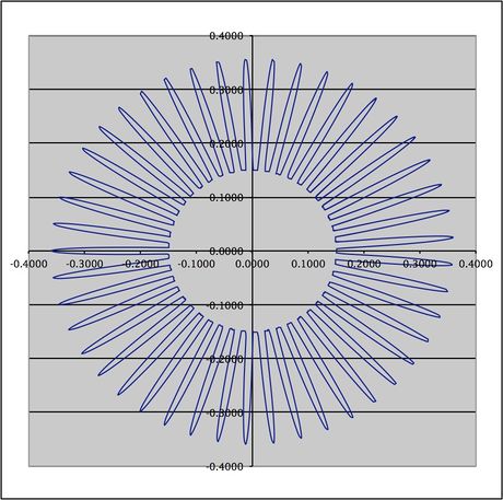
    24. Select C6:D2886 and chart them using a smoothed line scatter graph. Keep it off to one side, or at bottom -- my window is split at row 7 as per usual; you may prefer to work otherwise. The chart looks like this:
        How to Create the Idea of an Idea Image Picture 3
11. Save the Workbook. Enter the remaining Lookup Tables, starting with LOOKER on the Data worksheet:

    1. Edit Go To cell range  O6:O2886 and with O6 the active cell, enter 1. Do Edit Fill Series Columns Linear Step Value 1 OK. Select cell O5 and type LOOKER.
    2. Edit Go To cell Range P6:P2886 and with P6 the active cell, enter .125 and then do Edit Fill Down. Select P5 and type Std. 1/8th
    3. Edit Go To cell range Q6:Q2886 and with Q6 the active high-lighted cell, enter the formula, "=O6*$Q$35/$O$35" and do Edit Fill Down. Select cell Q35 and input .125; Select cell Q5 and type Relative. Select cell Q6 and do Insert New Comment and edit in "Original formula =O6*$Q$35/$O$35 with .125 in Q35."
    4. Edit Go To cell range O6:Q2886 and Insert Name Define LOOKER to range $O$6:$Q$2886. Format Cells Border (fire engine) Red Bold Outline.
12. Now enter the SpreadLooker table:

    1. Select cell U5 and input 1.
    2. Select cell W1 and type DIVIDED BY. Select cell W2 and Insert Define Name as DIVIDED_BY and Format Cells Border Outline Black.
    3. MODIFIED: Select cell W2 and input 1. Do Insert Comment and edit comment "Try .25 or .5 when Lookup Table fully operational -- playing with this idea -- not settled yet. Entering a 6 leads to beginning of chaos! Has to do with Phases? Inputting .6 in the current circumstances leads to rows>2880 but the design is not so great."
    4. Select cell U6 and input the formula, "=(6+AjRows/(Spheroids))/DIVIDED_BY". Do Insert New Comment and edit in "Original formula =(6+AjRows/(Spheroids))/DIVIDED_BY. So, in the case of 24 Spheroids and 2880 AjRows, 2880/24 = 120 + 6 = 126. The original Vlookup formula finds which row() it's currently in and compares it to this number, thus bracketing the data (spheroids) into groups (of rows)."
    5. MODIFIED: Select cell U4 and enter formula "=U6-6" w/o quotes. Do Insert New Comment and edit in "Original formula =U6-6." Insert Name Define Increment for cell $U$4. Do Format Cells Number Custom "Increment "0.0 and double click the U column header's right divider line to auto-adjust to fit. Format Font 14 red and Border Blue bold Outline.
    6. MODIFIED: Edit Go To cell range U7:U105 and with U7 the active high-lighted cell, enter the formula, "=Increment+U6" and do Edit Fill Down. Do Insert New Comment and edit in "Original formula =Increment+U6"
    7. Select cell V4 and type SpreadLooker. Format Cells Fill canary yellow Font fire engine Red Bold.
    8. Enter 1 into cell V5.
    9. MODIFIED: Edit Go To cell range V6:V105 and with V6 the active high-lighted cell, enter the formula, "=Spheroids-IF((Spheroids-(ROW()-5))>0,(Spheroids-(ROW()-5)),0)" and do Edit Fill Down. Do Insert New Comment and edit in "Original formula =Spheroids-IF((Spheroids-(ROW()-5))>0,(Spheroids-(ROW()-5)),0) which will progress in a step value of 1 until the number of Spheroids is reached and then repeat that number."
    10. Select cell W4 and type Spreader.
    11. MODIFIED: Edit Go To cell range W5:W105 and with cell W5 active and high-lighted, enter the formula, "=VLOOKUP(V5,Goal_Looker_Eggbasket,2)" and do Edit Fill Down. Do Insert New Comment and edit in "Original formula =VLOOKUP(V5,Goal_Looker_Eggbasket,2), i.e. it will look up the Spheroid number from column V here and then go on the Goal Looker worksheet's #2 B column of the Defined Range 'Goal_Looker_Eggbasket' there in cells A2:C102 matching that Spheroid number -- i.e. it will return a unique (random?) value per Spheroid for the number of Spheroids the user has input."
    12. Select cell X4 and type Eggbasket.
    13. MODIFIED: Edit Go To cell range X5:X105 and with cell X5 active and high-lighted, enter the formula,"=VLOOKUP(V5,Goal_Looker_Eggbasket,3)" and do Edit Fill Down. Do Insert New Comment and edit in "Original formula =VLOOKUP(V5,Goal_Looker_Eggbasket,3), i.e. it will lookup the Spheroid number from column V here and then go on the Goal Looker worksheet's #3 C column of the Defined Range 'Goal_Looker_Eggbasket' there in cells A2:C102 matching that Spheroid number -- i.e. it will return a unique (random?) value per Spheroid for the number of Spheroids the user has input. This (random?) value will be returned to Main X and Main Y."
    14. Edit Go To cell range U5:X105 and Insert Define Name  SpreadLooker to cell range $U$5:$X$105.
    15. MODIFIED: Do Format Cells Fill sky blue. Select cell U6 and do Format Cells Fill color rosy red and font red bold because the formula is different from the others in the column.
    16. Select cell range W5:X64 and Format Cells Number Decimal Places 2.
13. Activate or create a new worksheet Goal Looker if not already done.

    1. Input the Column Headings. A1: RANGE; B1: Pasted VAL; C1: EggBasket; D1: RandBetween; E1: Spiral. Select columns A:E and do Format Column Autofit Selection, Format Cells Number 2 decimal places OK.
    2. MODIFIED: Edit Go To cell range A2:C65 and Insert Name Define  Goal_Looker_Eggbasket  to cell range $A$2:$C$102.
    3. MODIFIED: Edit Go To cell range A2:A102 and with A2 the active high-lighted cell, input 1, then do Edit Fill Series Columns Linear Step Value 1 OK.
    4. MODIFIED: Edit Go To cell range D2:D102 and with D2 active, enter "=randbetween(60,78)/100" and Edit Fill Down. Your values will come out differently than mine. Copy the cell range and do Paste Special Values to cell B2.
    5. MODIFIED AGAIN: Edit Go To D2:D102 and with D2 the active high-lighted cell, enter the formula "=RANDBETWEEN(0,35)/100" and do Edit Fill Down. Copy these values and do Paste Special Values into cell range C2:C65 Do Insert New Comment into cell D2 and edit in "Original formula =RANDBETWEEN(60,78)/100 but =RANDBETWEEN(40,150)/100 also works just fine -- it just creates a larger spread of random numbers is all. Now is =RANDBETWEEN(0,35)/100".
14. Check for errors; there should be none except the planned approved ones mentioned herein for the top and bottom of Rose's X and Y columns. To get a good chart, columns E:N of the Data worksheet should generally be error-free. See the Warnings section below for help in errors reduction.

Explanatory Charts, Diagrams, Photos

1. (dependent upon the tutorial data above)

1. Create the Chart.

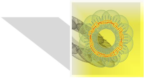
   1. MODIFIED: Activate Data worksheet and Edit Go To cell range H6:I2886. Either do Chart Wizard or select Chart on the Ribbon (activated in Preferences) and select All, Scattered, Smoothed Line Scattered. If using Chart Wizard, a new Chart worksheet will be created. Otherwise, copy or cut and paste the chart into the upper left corner of the Chart worksheet you created at the beginning, and hover the mouse over the lower right corner until it becomes a double-headed arrow and then use it to pull the chart into an expansion of a large Square. When I do it, sometimes it does not work right and it takes another column instead of column H. Click on the second standard ring series, or double-click until it appears in the formula bar and edit it until it reads as follows: =SERIES(,Data!$H$6:$H$2886,Data!$I$6:$I$2886,1). Edit the line of Series 1 to be solid and .5 point line weight and slightly yellowish Green in hue. It has no glow. This is the ring of 12 large spheres. Select Shadow and check it and set it to Perspective, black, size=100%, blur = 5 pt, distance - 0 pt, transparency = 53%.
   2. MODIFIED: On the Chart worksheet, do menu item Chart Add Data. In response to the Range request, activate the Data worksheet again and Edit Go To cell range J6:K2886.  When I do it, sometimes it does not work right and it takes another column instead of column J. Click on the second standard ring series, or double-click until it appears in the formula bar and edit it until it reads as follows: =SERIES(,Data!$J$6:$J$2886,Data!$K$6:$K$2886,2).  Format Selection solid and Line Weight 2 pt and Dark Dark Green from the color table, transparency 51%. This is the rose with the hole in it. Set Shadow to checked, perspective, 135 degrees, 100% size, 5 pt blur,  0 distance and transparency 53%. It has a yellow glow of 8 pt, 72% transparent, 0 soft edges pts.
   3. Any other series which Excel creates besides those in this description should be deleted by clicking on it and deleting it from the Formula Bar.
   4. MODIFIED: On the Chart worksheet, do menuitem Chart Add Data. In response to the Range request, activate the Data worksheet again and Edit Go To cell range E6:F2886. When I do it, it does not work right and it takes something instead of column E and F. Click on this next/center series3, or double-click until it appears in the formula bar and edit it until it reads as follows: =SERIES(,Data!$E$6:$E$2886,Data!$F$6:$F$2886,3). Set Glow to Yellow 5 pt, 0% transparency, no soft edges. Set Line to Fire Engine Red 0% transparency, smoothed line, 2pt line weight solid style.
   5. MODIFY? You may add the Eggies of Chart Series columns M and N if you prefer.
   6. MODIFIED: Format Selection of the Plot Area and set the Gradient to be Rectangular, From Upper left corner, Yellow on far left and Black at 62% on right. I have No Line, No Glow, and No Shadow set for the Plot Area, no Chart Titles, No Axes which are all controlled by Chart Layout (which appears on the Ribbon when you click on the Chart Plot Area).
   7. NEW: Chart Area: Line Auto, Fill is 70% yellow and the marker for  the medium grey is at far right of the gradient settings. Shadow is checked, perspective, 135 degrees, black, 78% size, 5 pt blur, 0 distance and 85% transparency.
   8. Copy the formulas  from A1:X105 to the Saves worksheet and then, below the formulas, paste them again, and then do Paste Special Values right over them. Then with the shift key held down, take a picture of the chart, Pasting Picture with the shift key depressed into the Saves worksheet under the data.
   9. Save the workbook.
2. How to Create the Idea of an Idea Image Picture 4
   Finished!

Helpful Guidance

1. Make use of helper articles when proceeding through this tutorial:

   1. See the article How to Create a Spirallic Spin Particle Path or Necklace Form or Spherical Border for a list of articles related to Excel, Geometric and/or Trigonometric Art, Charting/Diagramming and Algebraic Formulation.
   2. For more art charts and graphs, you might also want to click on Category:Microsoft Excel Imagery, Category:Mathematics, Category:Spreadsheets or Category:Graphics to view many Excel worksheets and charts where Trigonometry, Geometry and Calculus have been turned into Art, or simply click on the category as appears in the upper right white portion of this page, or at the bottom left of the page.