How to name, comment and protect cells in Excel

The following article shows you how to name, comment and protect cells in Excel.

1. Name the data cell.

- Normally, the data cell with the default name is the combination of the column and row order that makes up the cell. For example, cell B5 is named B5.

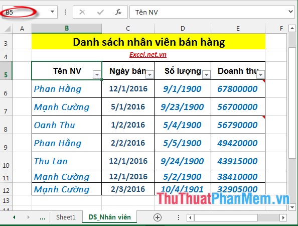
- To change the name of a cell, do as follows:

+ Click on the cell to be named -> in the formula bar enter the name in the Name Box field -> press Enter -> so the cell has been named:

2. Add notes to the data box.

Step 1: Click on the box you want to add notes -> Review -> New Comment:

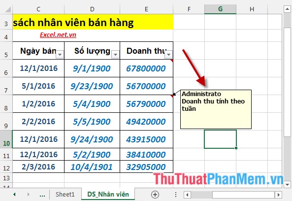
Step 2: A TextBox appears entering the text of the note:

- Cells with notes usually have small red triangle in the top right corner of the cell:

- When you move to the cell containing the note -> it is displayed:

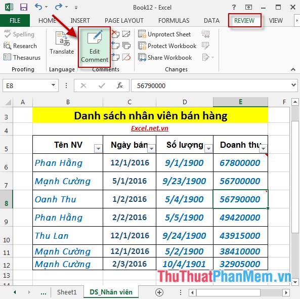
- In case you want to edit the note, do the following: Click on the cell containing the note -> Review -> Edit Comment:

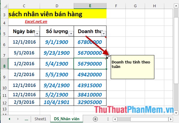
- After entering the note content, the results will be:

3. Protect data cells.

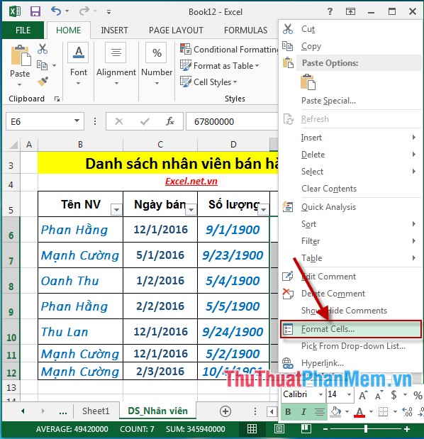
Step 1: Right-click the cell to be protected -> Format Cells:

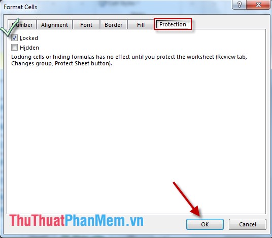
Step 2: The Format Cells dialog box appears -> select Tab Protection -> select Locked:

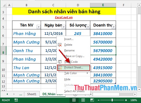
Step 3: Right-click the sheet name -> Protect Sheet to set password protection:

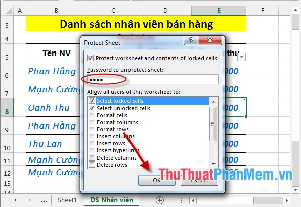
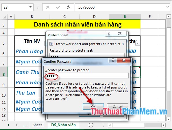
Step 4: A dialog box appears enter the password in the Password to unprotect sheet, can choose to add some features for users in the Allow all users of this worksheet to section -> select OK:

Step 5: A dialog box appears asking for password again -> retype the correct password -> click OK to finish.

- After setting protection, click the protected data box to edit the data -> Excel gives the following notice:

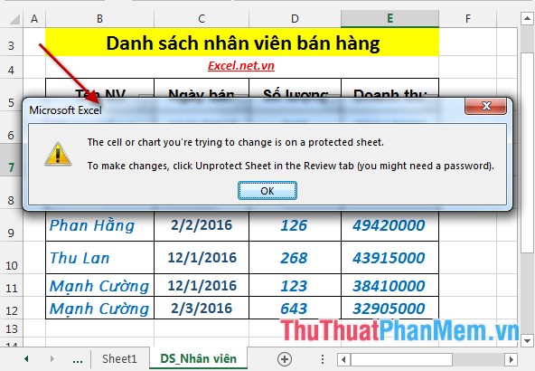
So your data is protected.

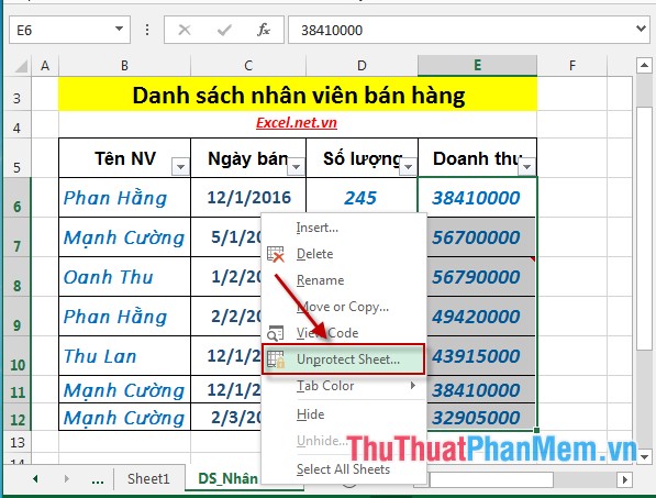
- In case you want to edit the data -> Unprotect data on the sheet by:

+ Right-click on the sheet name -> Unprotect sheet:

+ Enter the password you have set -> click OK.

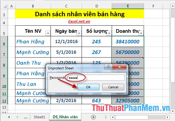
- After clicking OK you can edit your data arbitrary.

Above is a detailed guide on naming, annotating and protecting data cells in Excel 2013.

Good luck!