5 Hidden Functions in Google Sheets That Excel Doesn't Have

When you think of spreadsheets, Microsoft Excel is probably the first thing that comes to mind. It's a classic powerhouse, packed with features, powerful integration, and the ability to crunch massive amounts of data like a pro. For many, it's the de facto standard, and in many ways, that's still true. However, Excel doesn't do it all.

 

Many people use both apps regularly. Even though you rely heavily on Excel for heavy lifting, there are some Sheets functions that you'll miss every time you come back. If you're thinking about quitting Google Sheets and going back to Excel, it's worth knowing what you'll be leaving behind.

ISEMAIL and ISURL functions

Data validation made simple

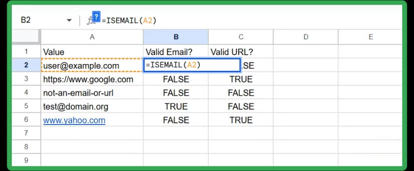
These two functions allow you to validate whether a string in a cell is a properly formatted email address or a valid URL . If you enter the following formula into a cell, Google Sheets will immediately return TRUE or FALSE depending on whether the text in cell A2 meets the criteria for a real email address:

 

=ISEMAIL(A2)

The ISURL function works similarly for web links.

At first glance, these functions may seem like small utilities, but they can save you a lot of time when working with customer data, signup forms, or marketing lists.

COUNTUNIQUE function

Count unique values ​​instantly

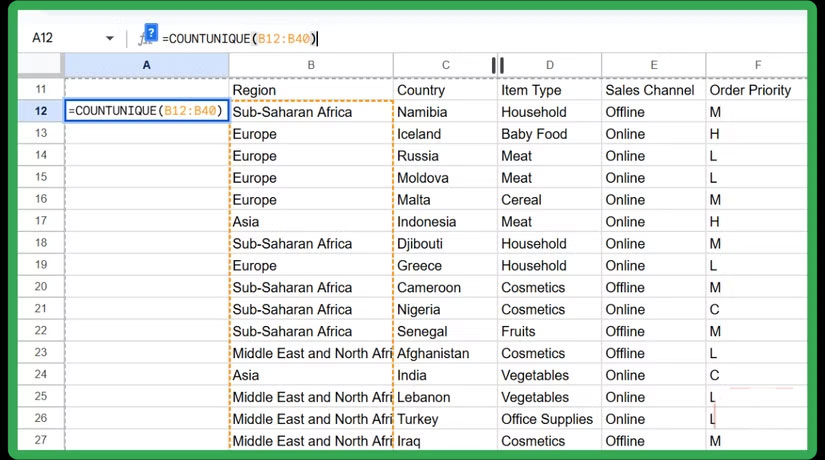
With this function, Google Sheets makes it easy to determine the number of distinct values ​​in a data set. By entering the following formula, you can calculate the number of unique items that appear in that range without any hassle:

=COUNTUNIQUE(A1:A100)

If your list contains apple, apple, banana, orange, orange , the result is 3. Each unique item will have a value, no matter how many times it appears.

You can use this function to count the number of unique customers in an order list, the number of unique product categories in inventory, or the number of distinct project codes in a dataset. Instead of manually sorting, filtering, or scanning through rows, you can count them directly in one step.

IMPORTFEED, IMPORTHTML, IMPORTRANGE, and IMPORTXML functions

Live data at your fingertips

 

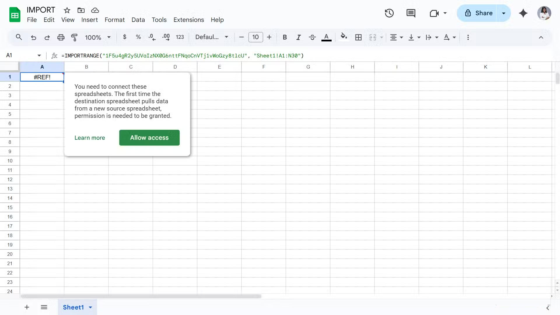
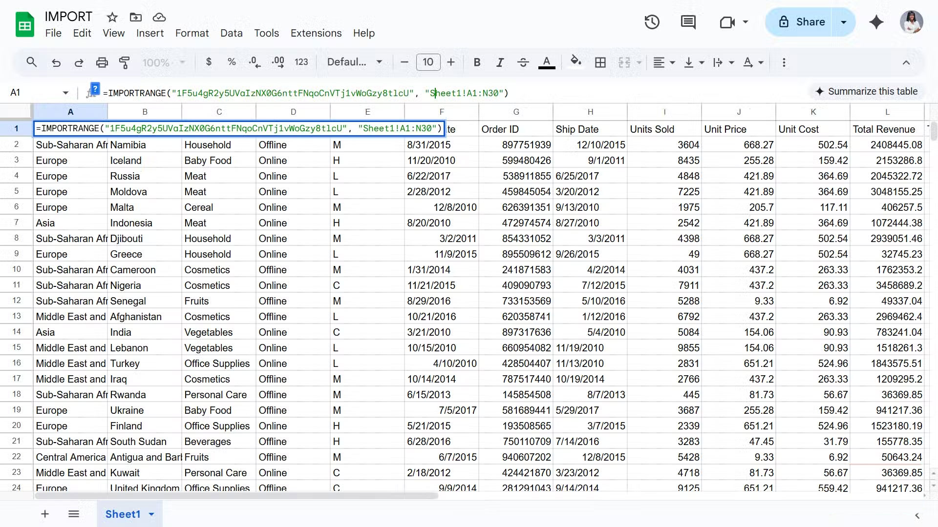
Another advantage of Google Sheets is the IMPORT function, which allows you to import external data directly into your spreadsheet with just one formula. Each function has its own role:

IMPORTRANGE	Get data from other Google Sheets
IMPORTHTML	Get a table or list from a website
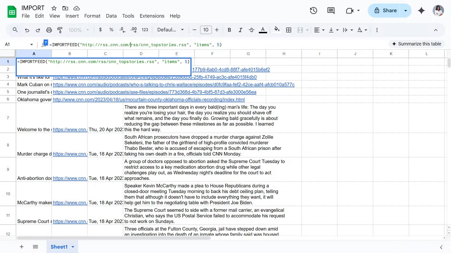
IMPORTFEED	Get RSS or Atom feed
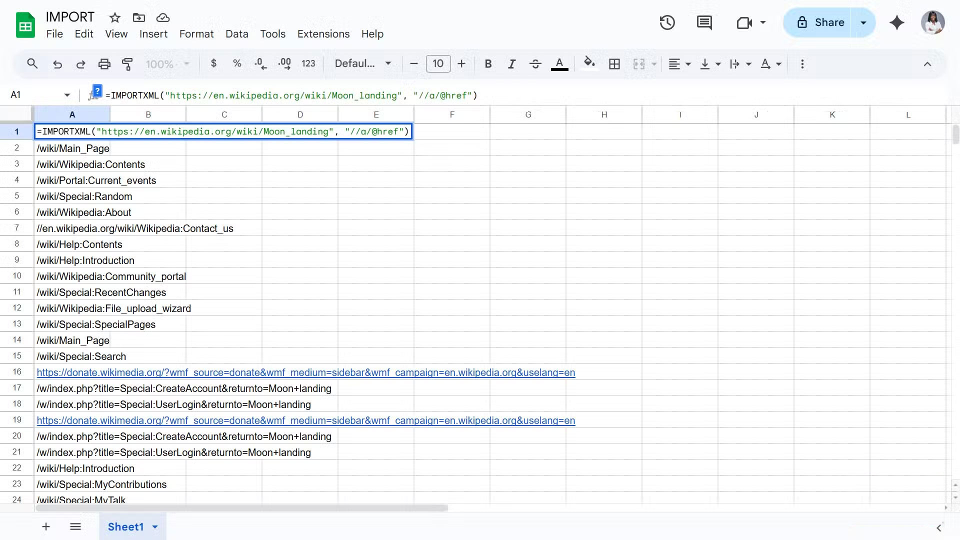
IMPORTXML	Handle more complex extraction operations, such as extracting specific web page components

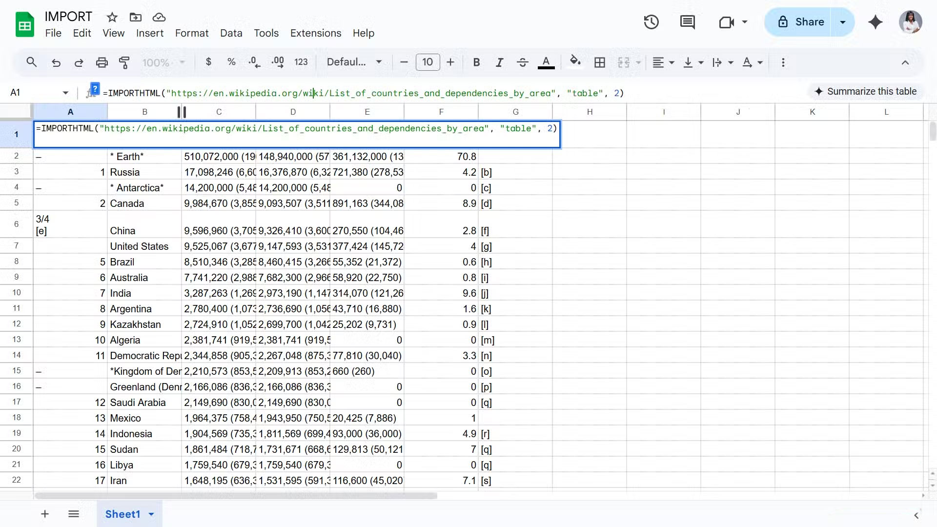
For example, you can paste this formula into a cell:

=IMPORTHTML("https://en.wikipedia.org/wiki/List_of_countries_and_dependencies_by_area", "table", 2)

This command tells Sheets to fetch the second table from the specified Wikipedia page and display it in your spreadsheet. Once you grant access, the data will be imported automatically and even updated when the source changes.

ARRAYFORMULA function

Truly adaptive dynamic arrays

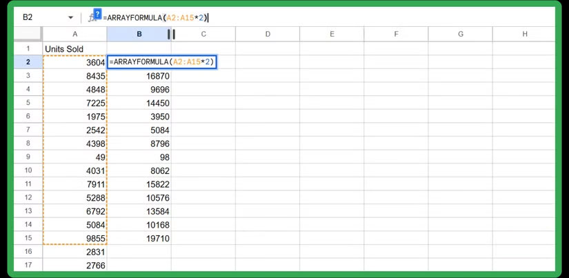
Instead of writing a formula in cell C1 and dragging it down hundreds of rows, you can write a single formula that autofills the entire column:

=ARRAYFORMULA(B1:B100*2)

This formula will instantly multiply every value in column B by 2, and the results will appear in the corresponding cells in column C.

This isn't to say that Excel doesn't have array formulas, but the approach has always been more complicated. First, older versions required the Ctrl + Shift + Enter method . You had to first select the range, enter the formula, and then confirm it by pressing the shortcut key. Then, Excel locked the formula in curly braces, creating a rigid structure that was difficult to edit or expand.

QUERY function

The Power of SQL in Spreadsheets

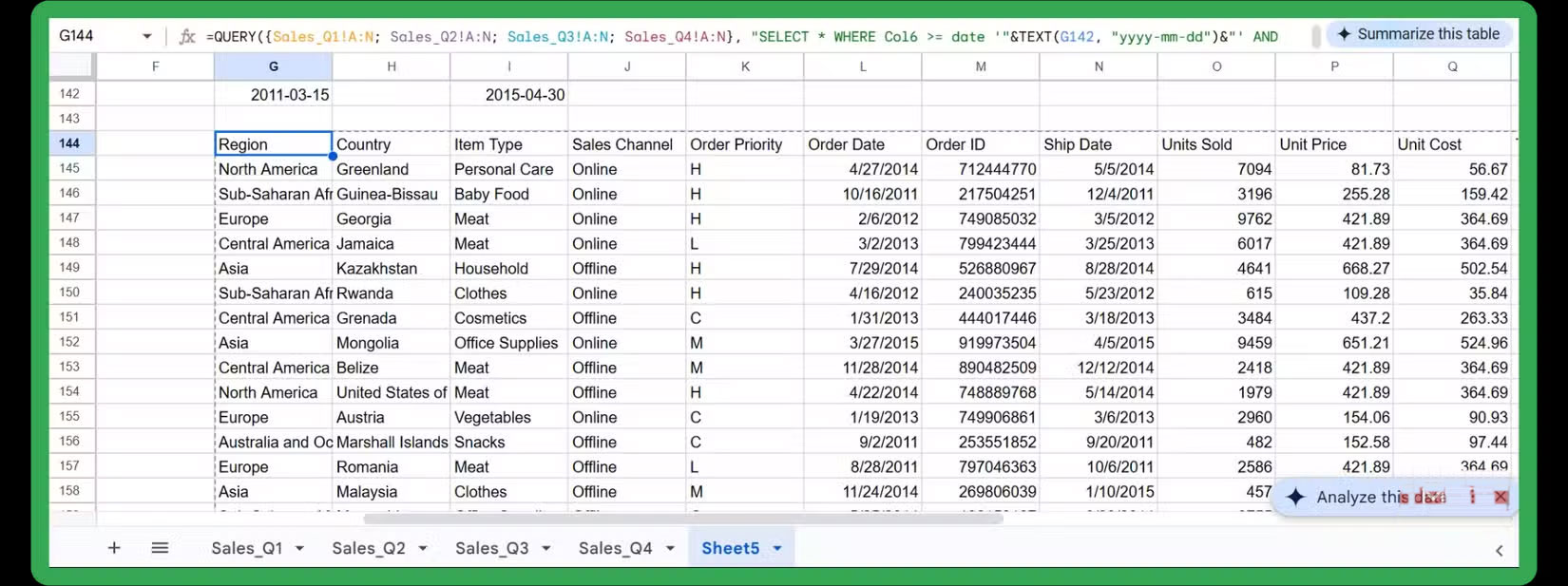
The QUERY function is one of the most powerful tools in Google Sheets. While not completely hidden, it is often overlooked because many people are unaware of its capabilities. In short, it brings SQL-style commands directly into your spreadsheet. You can filter, sort, group, and summarize data, just like you would with a database.

Imagine you want to group sales by region and sort the totals from highest to lowest. You could write something like this:

=QUERY(A1:G100, "SELECT C, SUM(D) WHERE G = TRUE GROUP BY C ORDER BY SUM(D) desc")

Simply put, this query takes data from columns A to G, checks a condition, groups rows by column C, sums column D, and sorts the results from largest to smallest—all in one formula.