9 basic Google Sheets functions you should know

Here are some simple Google Sheets functions.

1. SUM function

There is nothing more fundamental when working with numbers than adding up. Using the SUM function, you can sum multiple numbers, add the numbers in a cell, or use a combination of the two.

The syntax of the function is SUM(value1,value2,.) with value1 required and value2 optional.

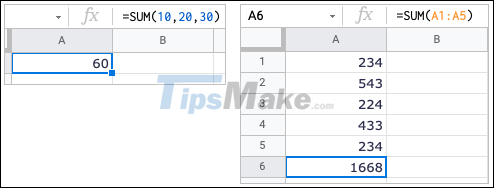
To sum the numbers 10, 20, and 30, you would use the following formula:

=SUM(10,20,30)

To sum the numbers in cells A1 through A5, you would use the following formula:

=SUM(A1:A5)

2. AVERAGE function

Maybe you need to know the average of the numbers in the range of cells. The AVERAGE function will help you do this.

Similar to how the average value is calculated in Excel, the syntax of the Google Sheets function is AVERAGE (value1,value2,.) with value1 required and value2 optional.

To find the average of the numbers 10, 20, and 30, you would use the following formula:

=AVERAGE(10,20,30)

To find the average of the numbers in the cell range A1 to A5, use the following formula:

=AVERAGE(A1:A5)

Tip: You can also view basic calculations without formulas in Google Sheets.

3. COUNT function

If you've ever had to count cells, you'll appreciate the COUNT function. With this function, you can count how many cells in a range contain numbers.

The syntax of the function is COUNT(value1,value2,.) where value1 is required and value2 is optional.

To count cells A1 through A5, you would use the following formula:

=COUNT(A1:A5)

To count cells A1 to A5 and D1 to D5, use the following formula:

=COUNT(A1:A5,D1:D5)

You can also count data that matches criteria using COUNTIF in Google Sheets.

4. NOW and TODAY functions

If you want to see the current date and time every time you open Google Sheets, you can use the NOW or TODAY function. NOW displays the date and time while TODAY shows only the current date.

The syntax for each function is NOW() and TODAY() with no required arguments, respectively. Simply enter one of the following into your worksheet to display the date and time, or just the date.

NOW() TODAY()

If you want dates to appear in a certain format, you can set the default date format in Google Sheets.

5. CLEAN function

When you enter data from another location into your worksheet, that data may include non-printable or ASCII characters such as spaces and carriage returns. The CLEAN function removes both visible and invisible characters.

The syntax is CLEAN(text) with the text part being required.

To remove non-printable characters from the text in cell A1, you would use the following formula:

=CLEAN(A1)

Note: Because this function removes both the characters you can and cannot see, you may not notice a difference in the resulting cell.

6. TRIM function

Another useful function for cleaning up sheets is TRIM. Just like in Microsoft Excel, this function removes spaces in a cell.

The syntax is TRIM(text) where the text can represent a cell reference or actual text.

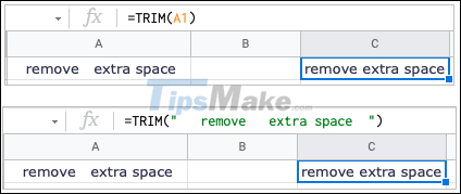
To remove spaces in cell A1, you would use the following formula:

=TRIM(A1)

To remove spaces from " remove extra space " use the following formula:

=TRIM(" remove extra space ")

7. CONCATENATE and CONCAT functions

To combine strings, text, or values, you can use the CONCATENATE and CONCAT functions. The main difference between these two functions is that CONCATENATE provides greater flexibility. For example, you can combine words and insert spaces between them.

The syntax for each function is CONCATENATE(string1,string2,.) and CONCAT(value1,value2) respectively where all arguments except string2 are required.

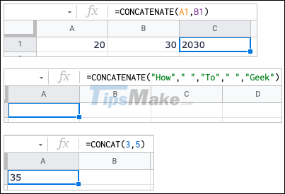
To combine the values ​​in cells A1 and B1, you can use the following formula:

=CONCATENATE(A1,B1)

To combine the words 'How', 'To' and 'Geek' with spaces, you would use this formula:

=CONCATENATE("How"," ","To"," ","Geek")

To combine the values ​​3 and 5, you can use the following formula:

=CONCAT(3,5)

8. IMAGE function

While Google Sheets offers the ability to insert images into cells, the IMAGE function gives you additional options to resize or set a custom height and width in pixels.

The function's syntax is IMAGE(url, mode, height, width) with the required URL and the other arguments optional.

To insert an image with a URL, you would use the following formula:

=IMAGE("https://tipsmake.com/template/en-cms-v2/images/logo.png")

To insert the same resized image with a custom height and width, use the following formula:

=IMAGE("https://tipsmake.com/template/en-cms-v2/images/logo.png", 4,50,200)

in this formula is a mode that allows custom size of the image to be 50 x 200 pixels.

Note: You cannot use SVG graphics or URLs for images in Google Drive.

9. ISEMAIL and ISURL functions

When importing data in Google Sheets, you may want to verify that it is the intended data. With ISEMAIL and ISURL, you can make sure the data is a valid email address or URL.

The syntax for each function is ISEMAIL(value) and ISURL(value) respectively, where you can use cell references or text. The validation result is displayed as TRUE or FALSE.

To check the email address in cell A1, you would use the following formula:

=ISEMAIL(A1)

To check the URL in cell A1, use the following formula:

=ISURL(A1)

To use text in a formula for an email address or URL, simply type it in quotes like this:

=ISURL("tipsmake.com")

Marvin Fry

Update 07 February 2022