How to use the QUERY function in Google Sheets

If you need to manipulate data in Google Sheets, the QUERY function can help you! It brings powerful database type search capabilities to spreadsheets, so you can look up and filter data in any format you want. The following article will show you how to use the QUERY function in Google Sheets.

Use the QUERY function

The QUERY function is not too difficult to master if you have ever interacted with the database using SQL. The format of a typical QUERY function is similar to SQL and brings the power of database search functionality to Google Sheets.

The format of a formula using the QUERY function is:

=QUERY(data, query, headers)

Replace 'data' with a range of cells (for example, 'A2: D12' or 'A: D' ).

The optional 'headers' argument sets the number of header rows to include at the beginning of the data range. If you have a title that spans two cells, like First in A1 and Name in A2 , then QUERY will use the content of the first two rows as the combined heading.

In the example below, a worksheet (called the 'Staff List' ) of a Google Sheets spreadsheet includes a staff list. It contains the name, employee ID number, date of birth, and whether they attended mandatory employee training.

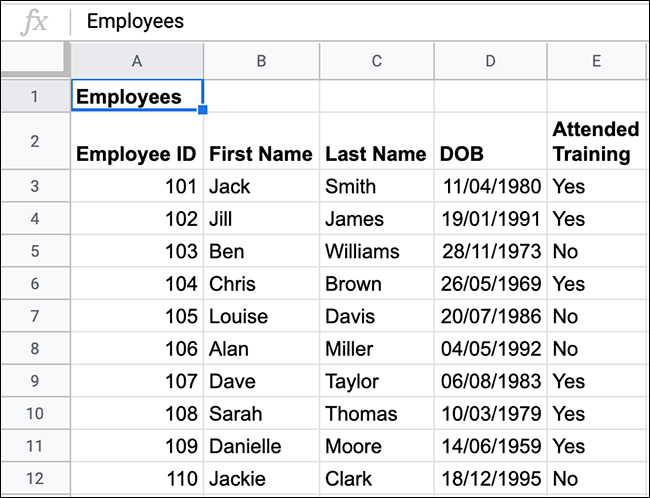How to use the QUERY function in Google Sheets Picture 1 Spreadsheet 'Staff List'

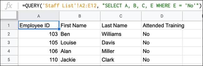
On the second worksheet, you can use the QUERY formula to get a list of all employees not attending the required training. This list will include the employee ID number, first name, last name, and whether they attended the training.

To do this with the data shown above, you can enter:

=QUERY('Staff List'!A2:E12, "SELECT A, B, C, E WHERE E = 'No'")

This queries data from the range A2 to E12 on the 'Staff List' page.

Like a regular SQL query, the QUERY function selects the columns to display ( SELECT ) and specifies the parameters for the search ( WHERE ). It returns columns A, B, C and E listing all matching rows, where the value in column E ( 'Attended Training' ) is a text string that says 'No'.

How to use the QUERY function in Google Sheets Picture 2 Column E ('Attended Training') is a text string that says 'No'.

As shown above, the 4 staff members on the list did not attend the training. The QUERY function provided this information, as well as matching columns to display employee names and ID numbers in a separate list.

This example uses a very specific data range. You can change to query all data in column A to E. This will allow you to continue adding new employees to the list. The QUERY formula you used will also update automatically whenever you add new employees or when someone joins a training session.

The exact formula to do this is:

=QUERY('Staff List'!A2:E, "Select A, B, C, E WHERE E = 'No'")

This formula ignores the original heading 'Employees' in cell A1.

If you add the 11th employee, not attending the training to the original list, as shown below ( Christine Smith ), the QUERY formula will also update and show the new employee.

How to use the QUERY function in Google Sheets Picture 3 The QUERY formula will update and display the new employee

Advanced QUERY formula

The QUERY function is very flexible. It allows you to use other logical operations (such as AND and OR ) or Google functions (such as COUNT ) as part of the search. You can also use comparison operators (bigger, smaller, etc.) to find values ​​between 2 numbers.

Use comparison operators with QUERY

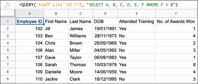
You can use QUERY with comparison operators (such as smaller, bigger or equal) to narrow and filter data. To do this, the article will add a column ( F ) to the 'Staff List' table , with the number of awards each employee has won.

Using QUERY, we can search all employees who have won at least one award. The format for this formula is:

=QUERY('Staff List'!A2:F12, "SELECT A, B, C, D, E, F WHERE F > 0")

This uses a comparison operator > to search for a value greater than 0 in column F .

How to use the QUERY function in Google Sheets Picture 4 Use comparison operators with QUERY

The above example shows the QUERY function returns a list of 8 employees who have won one or more awards. Out of 11 employees, 3 have never won an award.

Use AND and OR with QUERY

Nested logical operators like AND and OR work well in larger QUERY formulas, to add more search criteria to the formula.

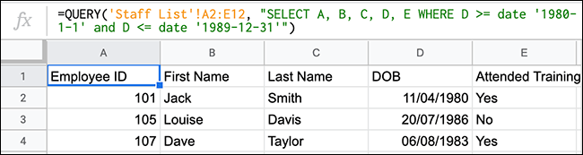
A good way to test AND is to look up data between two dates. If applied to the employee list example, the article can list all employees born between 1980 and 1989. This also takes advantage of comparison operators, such as greater than or equal to (> = ) and less than or equal to (<=).

The format for this formula is:

=QUERY('Staff List'!A2:E12, "SELECT A, B, C, D, E WHERE D >= DATE '1980-1-1' and D <= DATE '1989-12-31'")

This formula also uses the additional DATE function to accurately analyze the timestamp and search all birth dates between January 1, 1980 and December 31, 1989.

How to use the QUERY function in Google Sheets Picture 5 Birth dates between January 1, 1980 and December 31, 1989 will be listed

As stated above, 3 employees born in 1980, 1986 and 1983 meet these requirements.

You can also use OR to generate similar results. If using the same data, but converting dates and using OR , for example, all employees born in the 1980s can be excluded.

The format for this formula would be:

=QUERY('Staff List'!A2:E12, "SELECT A, B, C, D, E WHERE D >= DATE '1989-12-31' or D <= DATE '1980-1-1'")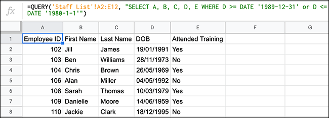

How to use the QUERY function in Google Sheets Picture 6 The remaining 7 were born before or after the excluded days

Of the original 10 employees, 3 were born in the 1980s. The above example shows the remaining 7 people who were born before or after the excluded days.

Use COUNT with QUERY

Instead of simply searching and returning data, you can also mix QUERY with other functions, like COUNT, to manipulate the data. Let's say, for example, we want to remove some employees from the list of people who have participated in the required training course.

To do this, you can combine QUERY with COUNT as follows:

=QUERY('Staff List'!A2:E12, "SELECT E, COUNT(E) group by E")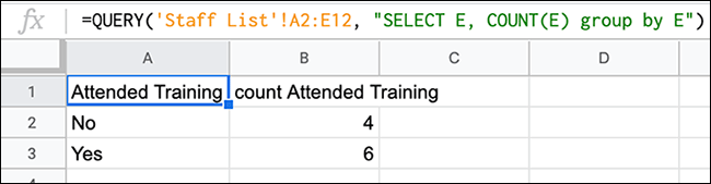

How to use the QUERY function in Google Sheets Picture 7 Use COUNT with QUERY

Looking at column E ( 'Attended Training' ), QUERY function used COUNT to count the number of times each value type (containing the text string Yes or No ). From the example list, 6 employees have completed the training and 4 have not.

You can easily change this formula and use it with other types of Google functions, like the SUM function.