5 Google Sheets formulas that will save you hours of tedious

Many people prefer Google Sheets , while others remain loyal to Excel. Still others fall somewhere in between, as they frequently use both spreadsheet tools. Depending on the specific task, one tool is often more suitable than the other.

If you use Google Sheets regularly, you'll learn that it can handle complex data manipulation quickly if you know which formulas to use and when. There are many formulas worth learning, but these five are the ones you'll frequently use whenever you open a Google Sheets file.

QUERY

Perform filtering, sorting, and summarizing in a single formula.

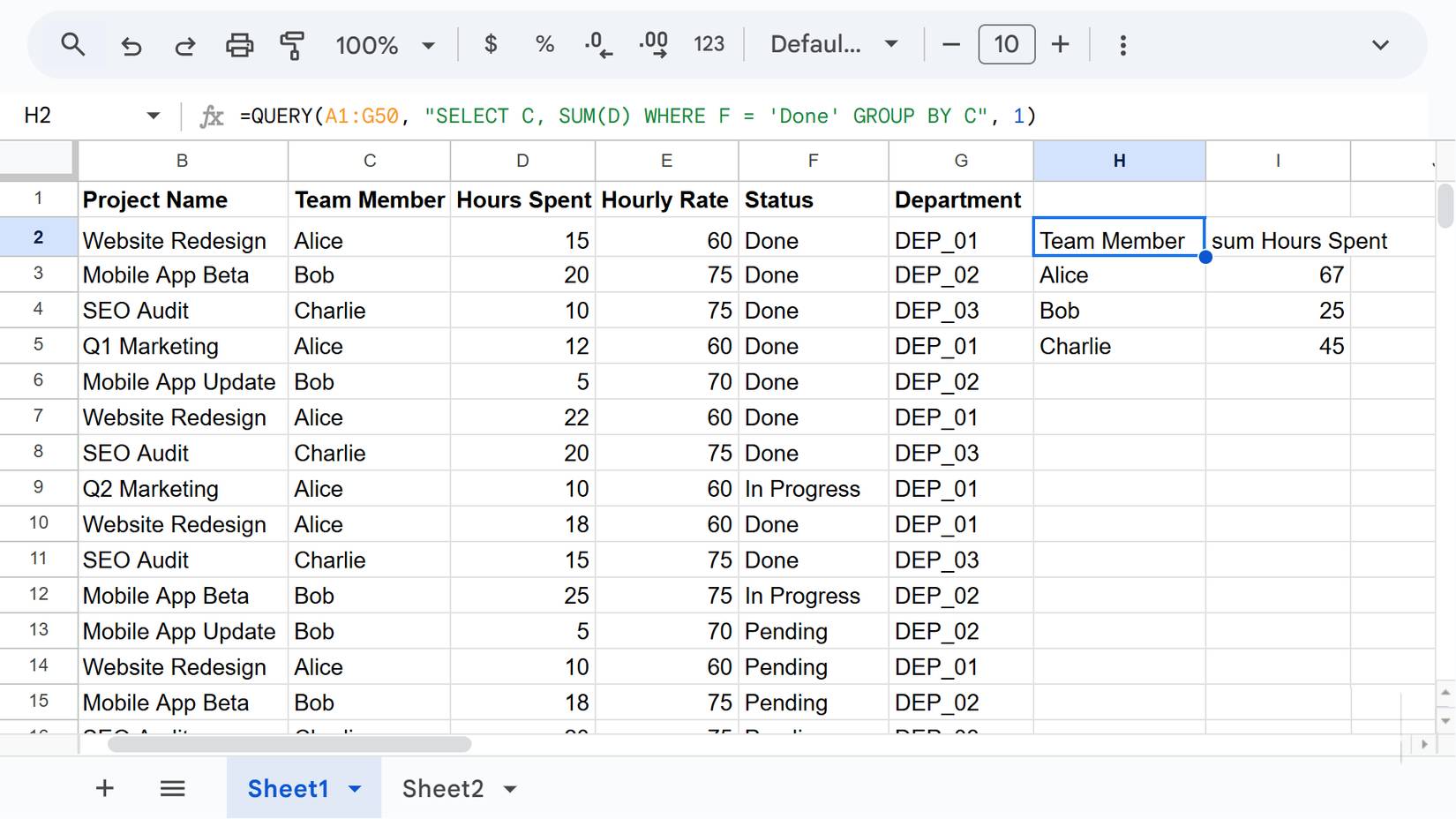
5 Google Sheets formulas that will save you hours of tedious work. Picture 1

If there's only one formula that saves you time, it's the one built with the QUERY function. This powerful formula allows you to run SQL- style queries in your spreadsheets, enabling you to filter, sort, and aggregate data precisely.

If you need to retrieve all completed tasks on your spreadsheet, group them by team member, and sum them up, the QUERY command can do all of that with simple syntax in just a few minutes:

=QUERY(data, query, [headers])

The ` data` argument here is the range you want to analyze, while the `query` argument is written in the Google Visualization API Query Language (essentially SQL Lite). The optional `headers` argument specifies the number of header rows in the dataset.

Now, in the query argument , you can use clauses such as select, where, group by, pivot, and limit , among many others. Google displays a complete list of supported clauses on the Google Charts website , which is worth bookmarking if you plan to use the QUERY command frequently.

IMPORTANCE

Retrieve data directly from other spreadsheets without copying and pasting.

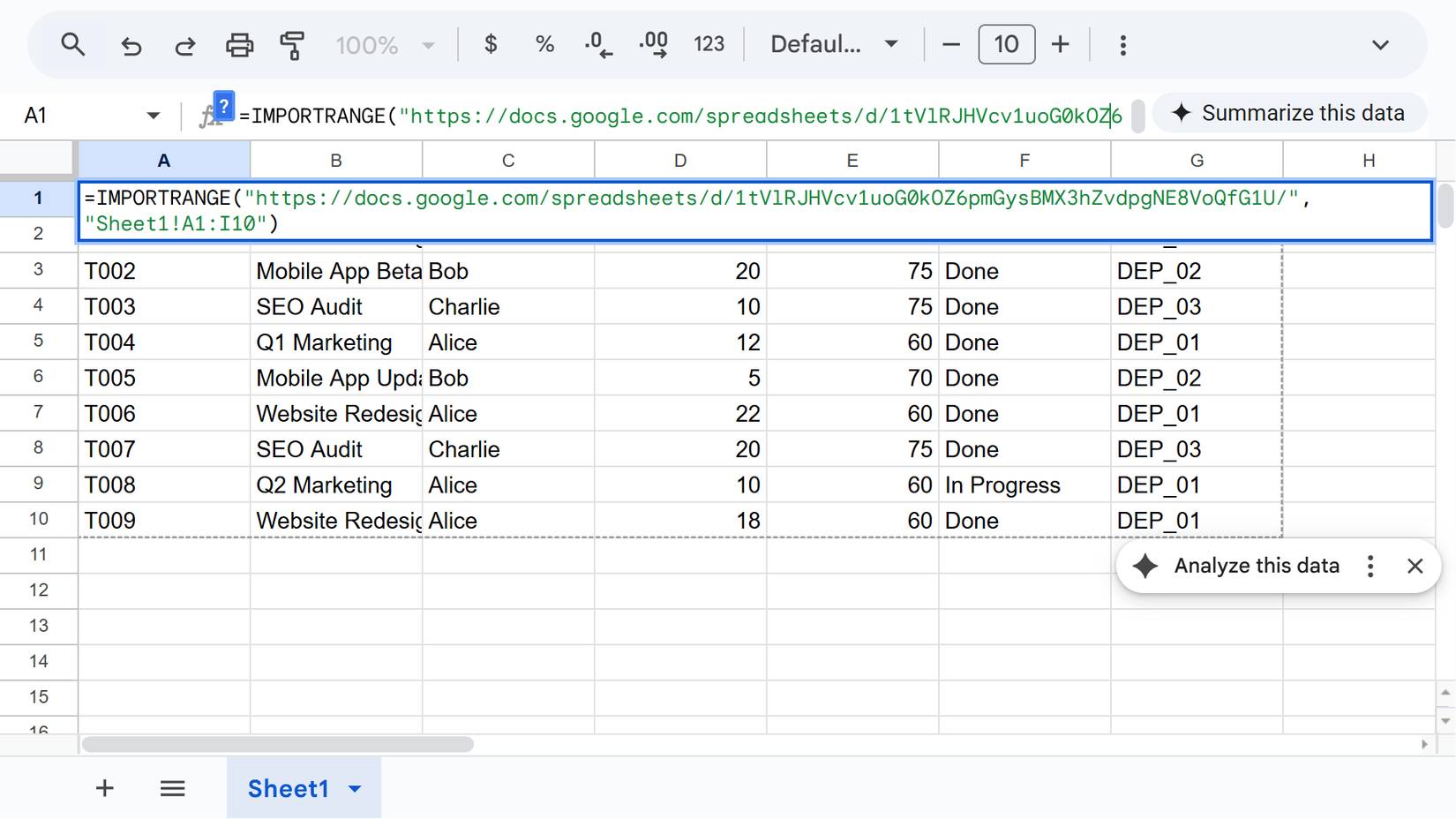
5 Google Sheets formulas that will save you hours of tedious work. Picture 2

When working with multiple spreadsheets, the alternative to using this function is often a combination of constantly switching tabs and excessive copy-paste operations. IMPORTRANGE eliminates that hassle by allowing you to pull data from any other Google Sheets spreadsheet directly into the spreadsheet you're working on with the following syntax:

=IMPORTRANGE(spreadsheet_url, range_string)

You simply need to enclose the URL of the source spreadsheet in double quotes, then specify the sheet name and range you want to import. A typical example might look like this:

=IMPORTRANGE("https://docs.google.com/spreadsheets/d/1tVlRJHVcv1uoG0kOZ6pmGysBMX3hZvdpgNE8VoQfG1U/", "Sheet1!A1:I10")

The first time you connect two spreadsheets, Google might prompt you to click Allow access , just to let you know that you're safe.

ARRAYFORMULA

Apply a formula to hundreds of rows automatically.

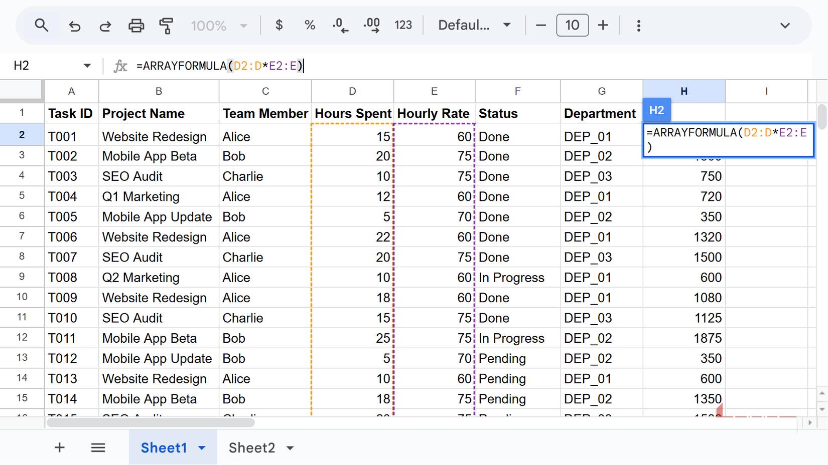
5 Google Sheets formulas that will save you hours of tedious work. Picture 3

The ARRAYFORMULA function applies a single calculation to the entire column at once, and it continues to run automatically as you add new rows. This makes a significant difference if you've ever had to drag a formula down hundreds or even thousands of rows just to update your spreadsheet.

The syntax is also quite simple:

=ARRAYFORMULA(array_formula)

Any calculations you place inside the function are applied to the entire range, meaning you can extend multiple standard formulas down a column without manually repeating them. Here's a simple example you can try:

=ARRAYFORMULA(D2:D*E2:E)

Instead of multiplying the number of working hours by the hourly rate for each individual row, this single formula will fill the entire column in one step.

LET

Write once, reuse the logic, stop repeating.

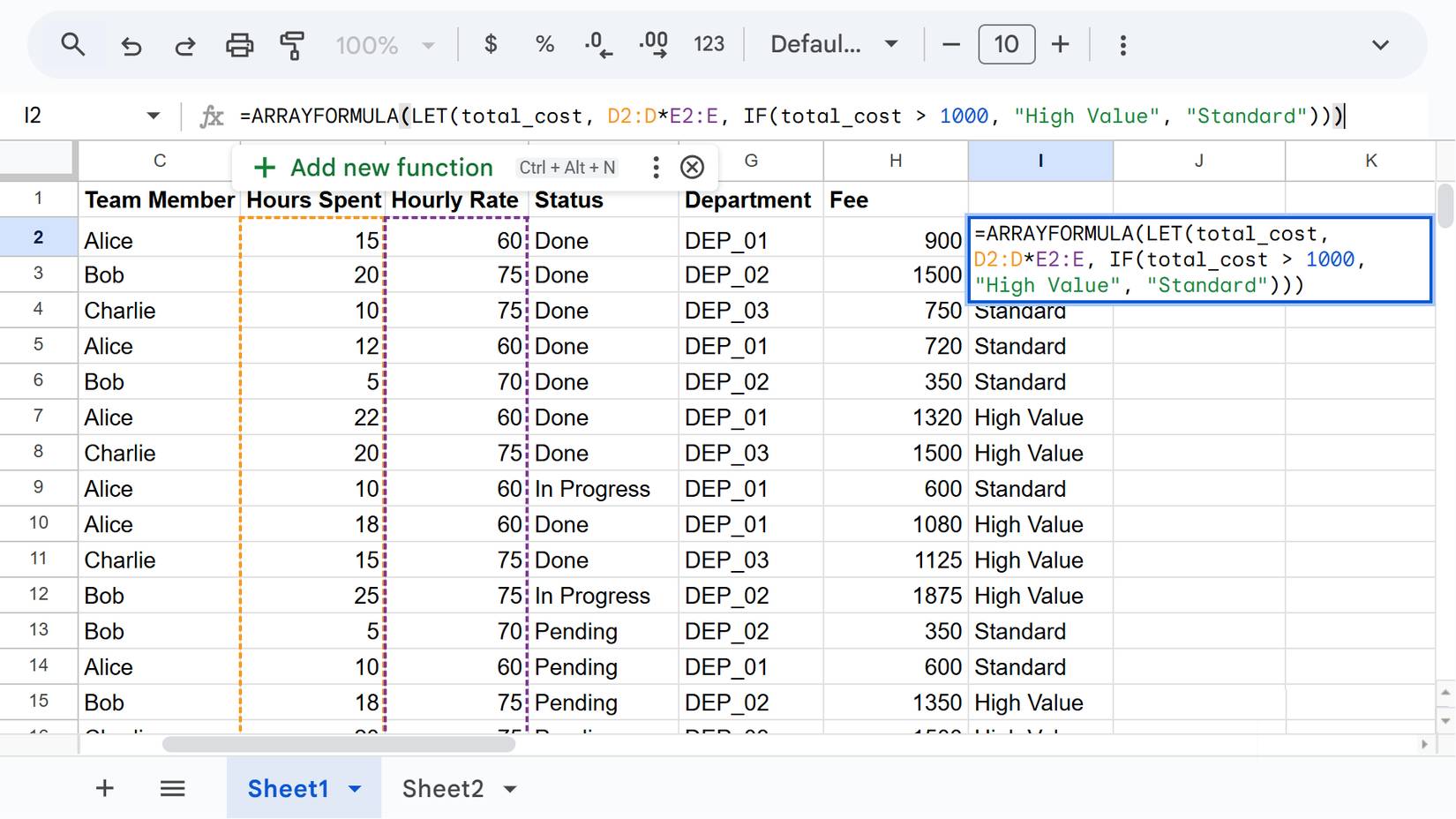
5 Google Sheets formulas that will save you hours of tedious work. Picture 4

People use LETs to name intermediate steps or results within complex formulas, so they don't have to repeat the same calculation multiple times. Once you define an expression in a formula, you can reuse that name throughout the entire formula, making it easier to read and maintain. That sounds confusing, but it becomes clearer when you see what the syntax looks like:

=LET(name1, value_expression1, [name2, …], [value_expression2, …], formula_expression)

This structure follows a simple pattern of name, value, name, value, etc., up to the last argument, which is the calculation you actually want Sheets to perform. In practice, this means you can create variables directly in your formulas, without needing helper cells or extra columns.

In all cases, Google Sheets evaluates each named expression only once, regardless of how many times it appears later in the formula or how many cells the formula fills. As a result, your spreadsheet runs faster, uses less memory, and is easier (and faster) to debug when problems occur.

XLOOKUP

Find accurate data without complex temporary solutions.

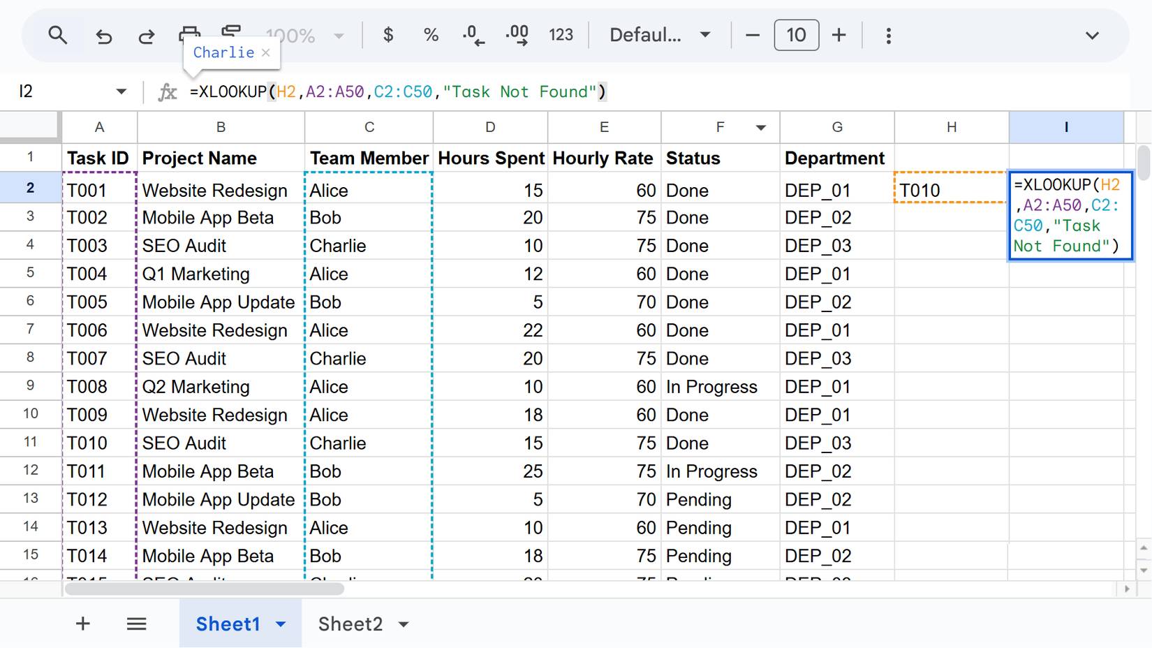
5 Google Sheets formulas that will save you hours of tedious work. Picture 5

XLOOKUP is a newer version of VLOOKUP, and it's the best way to perform searches in Google Sheets. The basic syntax looks like this:

=XLOOKUP(search_key, lookup_range, result_range)

With just these three arguments, you can perform quick and reliable searches in Google Sheets. There are also optional arguments to handle missing values, match types, and search direction, but even without them, XLOOKUP improves upon the old search functions. It can search in any direction instead of being limited to left-to-right, defaults to an exact match, and returns N/A when no value is found, which many consider a helpful error message.

These five formulas can help reclaim those precious minutes that Google Sheets often takes up in your day. Yes, it will take some getting used to and an initial investment of time to understand how each formula works.

However, once you master them, you can build spreadsheets that automatically handle tedious, repetitive tasks, allowing you to focus on data analysis, which is the most important thing.