Simple Power Query Commands That Save Hours Cleaning Up Excel Data

Cleaning up data in Excel , especially for multiple workbooks, is one of the most frustrating tasks any Excel user faces. But with Power Query, it becomes even more fun.

 

Split cells with delimiter

Easily split data into columns

A common problem when cleaning up an Excel spreadsheet is that data that should be split into two columns is merged into one. See the screenshot below, where the Order ID column also has the customer name.

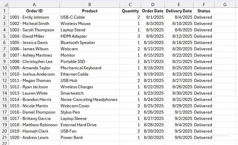
We'll split this column in Power Query with a delimiter, a character or symbol (such as a comma, space, or hyphen) that separates data in a cell. The delimiter is a hyphen or dash (-) that separates the order ID from the customer name in the example above.

 

Let's say you have this worksheet saved somewhere on your computer. To import, select the Data tab and click Get Data -> From File -> From Excel Workbook in the Get & Transform Data group of commands on the ribbon.

From there, navigate to the file location, select it, and click Import . In the Display Options on the left, select the sheet with the data and click Transform Data . Note that this is just one way to import data into the editor—the options will vary depending on where you got your data.

Except for the day

Determine the exact date difference

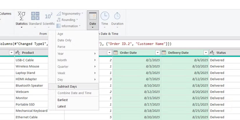
Continuing with the example table above, we can also perform various calculations on columns in the Power Query editor. Let's take this opportunity to add additional columns for certain calculations. The most common way people do this is to determine the difference between dates.

Here, for example, we want to find the number of delivery days for orders, so we need to subtract the delivery date from the order date. To do that, select the Delivery Date column , press Ctrl , then select Order Date (note the order of selection). Next, select the Add Column tab and click Date -> Subtract Days in the From Date & Time group of commands on the ribbon.

Filter errors

Make sure you only see the affected rows

Power Query doesn't have an easy way to filter to only show rows with errors. These rows can be a headache if they're in a file with hundreds or more rows.

 

Suppose you know that the Order Date column has errors and want to manually fix them before loading the data into Excel. You can create a filter to show only the affected rows.

Select the Add Column tab and click Custom Column in the General command group of the ribbon. In the Custom column formula text area , enter the following formula and click OK :

try [Order Date]

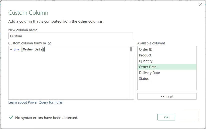
Power Query will add a new column called Custom , and the rows will have a value of TRUE if there is an error or FALSE if there is no error. Now, do the following:

1. Click the arrow icon to the left of the Custom column .
2. Uncheck all items except Has Error .
3. Click OK .
4. Click the arrow icon next to the Custom column again.
5. Uncheck False .
6. Click OK .

Unpivot data

Data analysis support

Pivoted data is data that is structured in a wide format, with values ​​spread across multiple columns. This can make it difficult to analyze the data when using Pivot Tables in Excel.

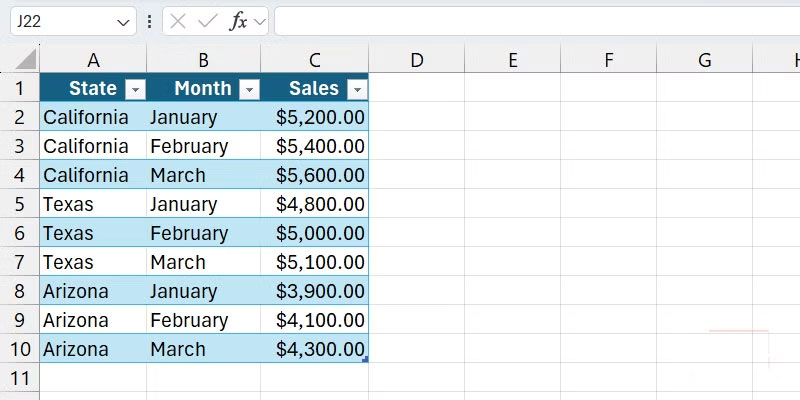
Take a look at the screenshot of the table below showing sales data by 3 states. Since months are a category, they should actually be arranged in rows instead of columns to aid in data analysis.

 

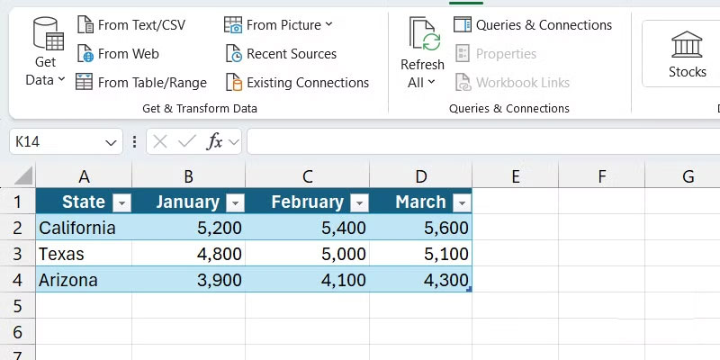
To fix this, we need to un-axis the data, which means the data needs to be reshaped into a tall format. Basically, the states, months, and sales need to be placed on separate rows.

Doing this manually would involve a lot of copying and pasting, manually aligning values, and making sure there are no errors. But Power Query can make this easier.

A simple query with huge impact

It's no exaggeration to say that Power Query will make you look forward to cleaning up your Excel data. This is especially true because you can create an automated process to clean multiple worksheets in the same way. And, as you can see, you can do a lot with just a few simple commands.