7 ways to clean up data in Microsoft Excel

Spelling errors, extra spaces, duplicates, formula errors, and blank cells can all cause trouble when parsing spreadsheet data. To clean up your Microsoft Excel spreadsheet, try one or more of the following ways to process the data.

1. Remove extra whitespace

Whether the word is entered or mistyped, you may have extra space in your data. This can include spaces at the beginning of cells, spaces at the end of cells, or miscellaneous spaces between words or values. While they may not seem important, you can easily run into problems filtering, sorting, or generating data.

There are two simple ways to remove extra spaces in your Excel worksheet: the TRIM function and the Find and Replace tool.

Using the TRIM . function

The TRIM function in Excel works especially well for removing spaces from your data. The formula's syntax is simply TRIM(text). Enter a cell reference or text for the argument.

Using the Find and Replace tool

If whitespace is scattered across the worksheet, you may want to use Excel's Find and Replace tool instead of the TRIM function. With this method you can remove all or some specific spaces.

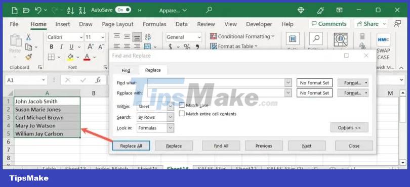
1. Go to the 'Home' tab, open the 'Find & Select' drop-down menu in the Editing section and select 'Replace'.

2. In the Find and Replace box that appears, use the 'Find what' box to enter a space if you want to remove all or the exact number of spaces you want to remove.

3. In the 'Replace with' box , enter nothing if you want to remove all spaces or the exact number of spaces you want to keep.

4. Select 'Replace All' to remove extra spaces and you'll see your sheet update immediately.

2. Remove non-printable characters

Non-printable characters are similar to extra spaces. These are the first 32 characters, including zeros, in the 7-bit ASCII code for things like nulls, headers, form feeds, carriage returns, and unit separators. Like spaces, these characters can cause problems when calculating formulas, sorting, or filtering in your Excel worksheet.

Conveniently, you can use a simple function to remove non-printable characters in Excel. This function is called CLEAN and the syntax of the formula is CLEAN(text), where you can enter text or cell references for the argument.

This example has non-printable characters CHAR(10) at the beginning and end of the formula in cell A1.

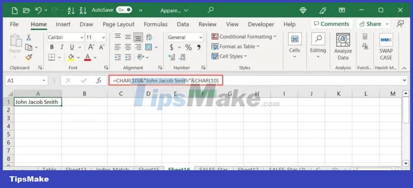
Use this formula to remove them:

=CLEAN(A1)

You can also enter text as part of the CLEAN function. Use the following formula if you want to replace existing text with more compact text.

=CLEAN(CHAR(10)&"John Jacob Smith"&CHAR(10))

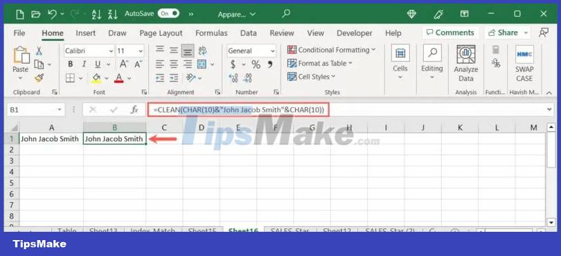
Non-printing characters are removed, leaving only text.

3. Delete empty rows

If you have blank rows in your worksheet, these can take up much-needed space for the actual data. You can remove blank rows in Excel with just a few steps and reclaim space in your worksheet.

Refer: How to add rows, delete rows in Excel for details on how to do it.

4. Find and remove duplicate data

Duplicate data is something that you might want to remove in your Excel worksheet. It could be a customer name, email address, phone number, or something like that.

There are several ways to find and remove duplicate data in Microsoft Excel and you can see the tutorial: How to remove duplicate data and content in Excel for different methods.

5. Delete Format

If more than one person is working on a worksheet or copying and pasting data from another location, the document can have more formatting that you don't need. This can include bold fonts, fills, or borders. Fortunately, you don't have to change every cell, row, or column. You can remove formatting in your worksheet with one click.

Note that if you set up conditional formatting in your worksheet, removing the formatting as explained here will also remove it.

1. Select the range of cells that contain the formatting you want to remove. The example applied bold, color, and italics to the text along with a fill and border color.

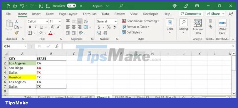
2. Go to the 'Home' tab, open the 'Clear' drop-down menu and select 'Clear Formats'.

3. You should see all formatting in those cells disappear.

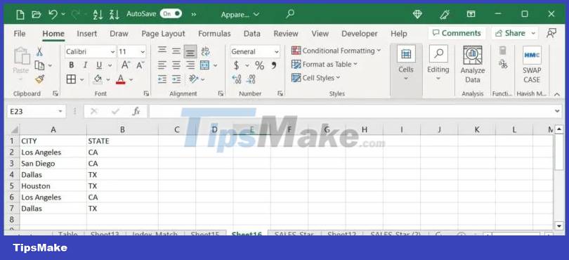
6. Convert text to columns

When you get data from another source, it's not always presented the way you want it to. You may have rows with data that needs to be placed in separate cells within columns. You can convert this text into columns in just a few steps to make it easier to work with.

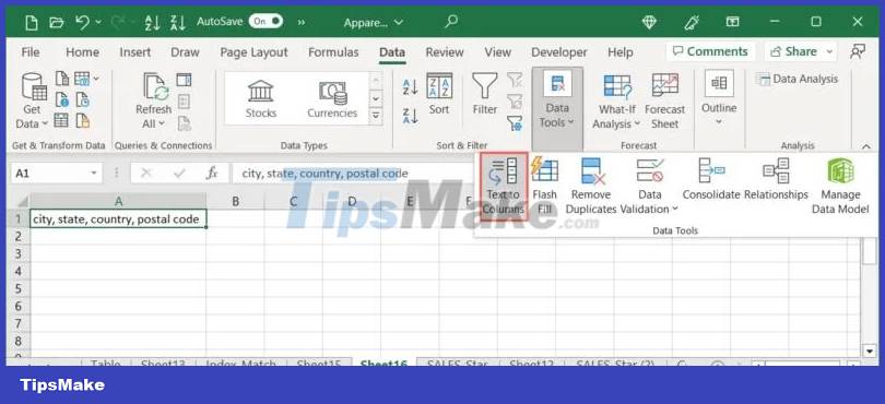
1. Select the cells you want to convert, go to the 'Data' tab and select 'Text to Columns' in the Data Tools group.

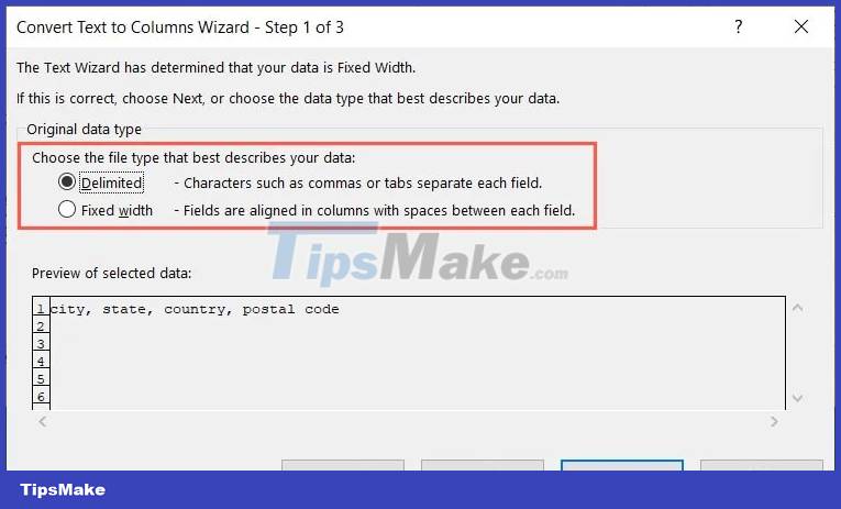
2. When the Convert Text to Column Wizard opens, take a few steps to convert your data based on its current state and how you want to display it. Start by selecting 'Delimited' or 'Fixed width'. Excel gives you suggestions based on your data, but you can choose whichever option works best. Click Next .

3. Depending on the option you choose in the first step, you will see the corresponding second step. For example, if you select Delimited data , you can select the separator, and if you select Fixed data , you can adjust the column width. Click Next.

4. Select a data format for the column, such as text or date, and enter a destination for the converted data. Click 'Finish'.

5. You'll see your text converted into columns, ready for you to work on.

7. Mark errors

Although Excel does a good job of pointing out errors in cells, such as errors in formulas, you may not notice these errors if you have a long workbook. With conditional formatting, you can highlight errors to make them easier to see and correct.

1. Select the entire sheet by clicking the 'Select All' button (triangle) at the top left of the sheet. If you only want to check certain cells, select those.

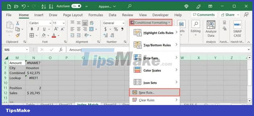
2. Go to the 'Home' tab, open the 'Conditional Formatting' drop-down menu in the Styles group and select 'New Rule'.

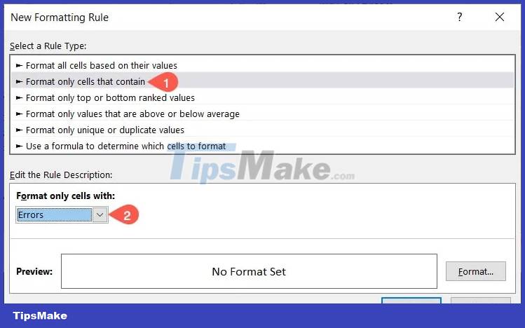
3. When the New Formatting Rule window opens, select 'Format only cells that contain' at the top and 'Errors' in the drop-down list at the bottom.

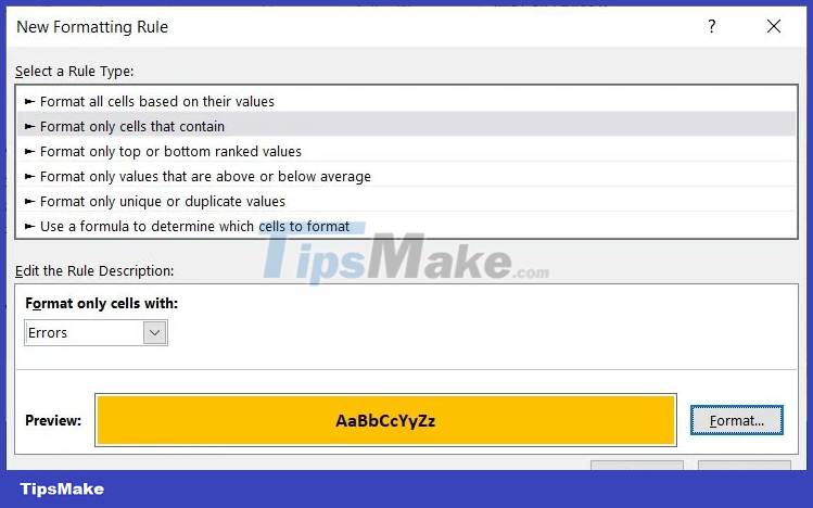
4. Click the 'Format' button to select the format you want to apply. You can do things like colorize cells, bold text, or add bold borders. Select 'OK' after you set the format.

5. You will see a preview of your selection at the bottom of the New Formatting Rule window . Click 'OK' to save and apply the rule.

6. When viewing the selected worksheet or cells, you will see the errors appear. After you correct the error, the formatting will disappear and you can move on to the next error.

Kareem Winters

Update 24 July 2023