Learn about XMATCH: Excel function is much smarter than VLOOKUP

VLOOKUP used to frustrate people with its rigid limitations and cumbersome syntax. But not anymore. There's an Excel function that can handle lookups in all directions and provides exact match control.

 

XMATCH works in any direction you want

The most annoying thing about VLOOKUP is that it requires a left-to-right search. If your lookup column isn't on the leftmost side of the range, you're stuck. You have to rearrange your data or find a workaround. Rearranging your spreadsheet just to get VLOOKUP to work properly can be time-consuming.

Excel's XMATCH function eliminates this headache. Unlike the rigid structure of VLOOKUP, XMATCH searches any array in any direction. You can search for data to the left of the lookup column. You can also search vertically down a column or horizontally across a row; XMATCH handles both with ease.

 

Here is the basic syntax:

=XMATCH(lookup_value, lookup_array, [match_mode], [search_mode])

Let's analyze these parameters:

1. lookup_value : The value you are looking for.
2. lookup_array : Search range.
3. match_mode : The level of precision required for the search results (0 is exact, -1 is exact or next smallest, 1 is exact or next largest).
4. search_mode : Search direction (1 is from start to end, -1 is from end to start, 2 is binary search).

Here's a real-world example from an employee database. Let's say you need to find what department "Kristen Tate" works in, but the employee name is in column D and the department is in column B. With VLOOKUP in an Excel spreadsheet, this setup would force you to rearrange the data because you can't look to the left.

But you can use the XMATCH function to return her position in the name column as shown in the following formula:

=XMATCH("Kristen Tate", D:D, 0)

 

It changed the workflow because you no longer had to count columns. With VLOOKUP in Excel, you had to keep counting to determine the column index number. If you added a new column to your data, your formula would suddenly fail because the index number changed.

 

XMATCH gives you more control over matching

VLOOKUP's matching options are limited to exact or approximate matches - that's it. If your data isn't perfectly clean, you'll have to spend time cleaning up a messy Excel spreadsheet before you can start your lookup.

XMATCH makes this easy with the match_mode parameter. Setting this to 0 for exact matches, just like VLOOKUP's FALSE parameter. But this is where things get interesting. You can use -1 to find an exact match or the next smallest value, and 1 to find an exact match or the next largest value.

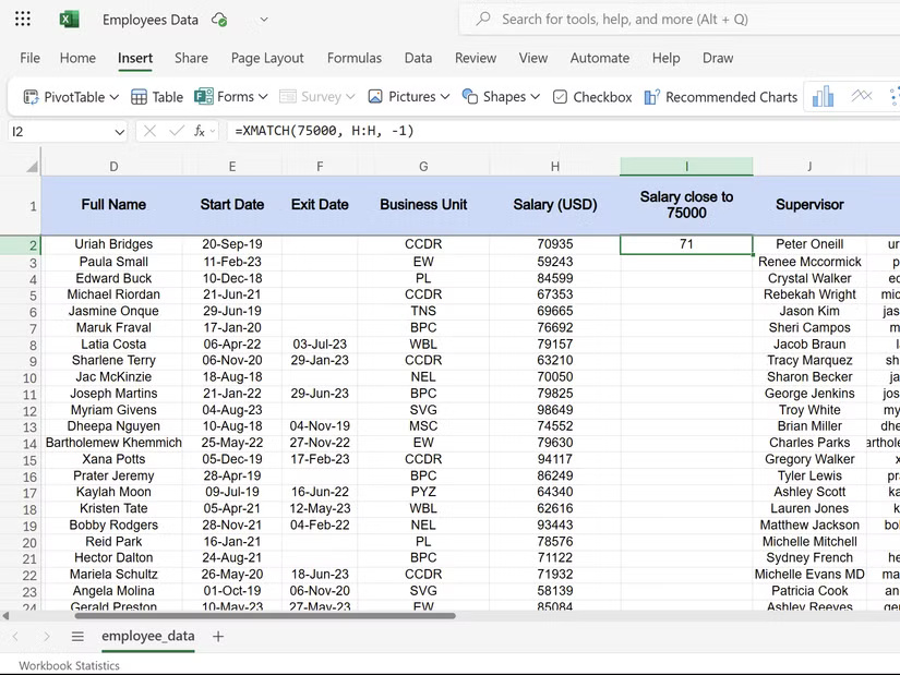
Consider the salaries in the employee dataset. To find the employee with the closest salary but not exceeding $75,000, you would use:

=XMATCH(75000, H:H, -1)

This formula returns the location of the highest salary from column H that does not exceed your target value - something VLOOKUP has trouble with unless the data is perfectly sorted.

 

The search_mode parameter adds an extra layer of control. While 1 searches from start to finish (default), -1 searches from end to start. This is important when you have duplicate values and need the most recent entry.

For example, if "John Smith" appears multiple times in column D of the data set, we can use the following formula to find his last occurrence.

=XMATCH("John Smith", D:D, 0, -1)

Understanding these parameters will help you look up data more efficiently. This level of control means fewer auxiliary columns and data manipulations. Your formulas become more powerful and your spreadsheets become cleaner.

XMATCH goes perfectly with INDEX

XMATCH becomes even more useful when you combine it with the INDEX function . While XMATCH finds the position, INDEX retrieves the actual value from that position. This is one of those Excel functions that is useful for quickly looking up data, but when combined together, they create a more flexible lookup combination.

Here is the basic syntax when you combine the two:

=INDEX(return_array, XMATCH(lookup_value, lookup_array, [match_mode]))

This combination eliminates the column counting nightmare of VLOOKUP. Instead of having to remember that salary is the 8th column, you can just specify the salary column directly. So you won't run into formula errors when adding or removing columns.

Let's say you need to find Kristen Tate's department from employee data using INDEX and XMATCH:

=INDEX(R:R, XMATCH("Kristen Tate", D:D, 0))

The above formula reads naturally and returns a value from column R at the position where "Kristen Tate" appears in column D.

 

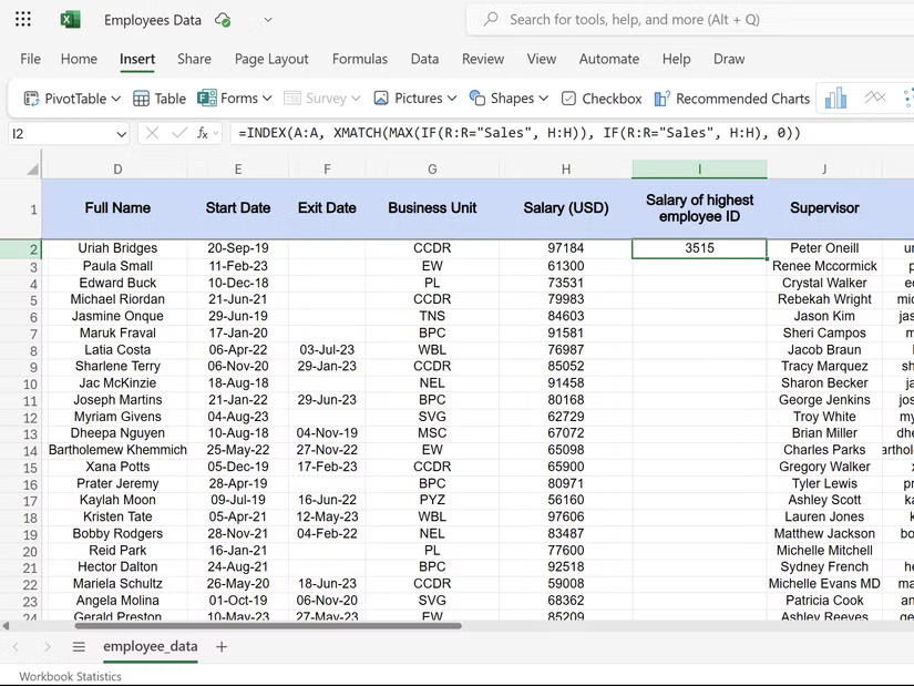
This combination also handles complex lookups, such as when you need the salary of the employee in the Sales department with the highest employee ID:

=INDEX(A:A, XMATCH(MAX(IF(R:R="Sales", H:H)), IF(R:R="Sales", H:H), 0))

This array formula finds the largest employee ID in the Sales department, then returns that person's salary. If you tried to do this with VLOOKUP, you would need multiple support columns and other workarounds.

XMATCH has completely replaced VLOOKUP in my workflow. Its directional flexibility, precise matching control, and easy INDEX integration make it the lookup function I've always needed. Once I've experienced this level of control, going back to VLOOKUP seems impractical.