How to combine Vlookup function with If function in Excel

Vlookup function and If function are important and basic functions in Excel. When combining these two functions, users can use in many calculations, statistics of different data such as showing employee information when just pressing the code. In this article we will show you how to set conditions to filter values, by combining the Vlookup function with the If function.

With certain conditional statistics and require users to fill in information based on that condition, you can use the Vlookup function with the If function, as in the rating table. The following example will help you better understand how to use the Vlookup function and If function to filter conditional values.

1. How to automatically display names when entering code in Excel
2. How to combine Sumif and Vlookup functions in Excel

How to use Vlookup function with If function

This is the student's test results and pass or score table. We have benchmarked each test block to see if students have enough passing grades, or fail. You need to enter test results for each student.

How to combine Vlookup function with If function in Excel Picture 1

The If function will look for results that are satisfied with the benchmark, thereby giving a conclusion of passing or failing. Then combine with the VLOOKUP function to filter the values ​​that satisfy each student. Finally, the two functions will produce the search results.

Vlookup function will have a formula:

1. VLOOKUP (lookup_value, table_array, col_index_num, [range_lookup])

If function has a formula:

1. IF (Logical_test, Value_if_True, Value_if_False)

Formula when nested Vlookup function and If function together

1. IF (Logical_test> = Vlookup (lookup_value, table_array, col_index_num, [range_lookup]), Value_if_True, Value_if_False)

Step 1:

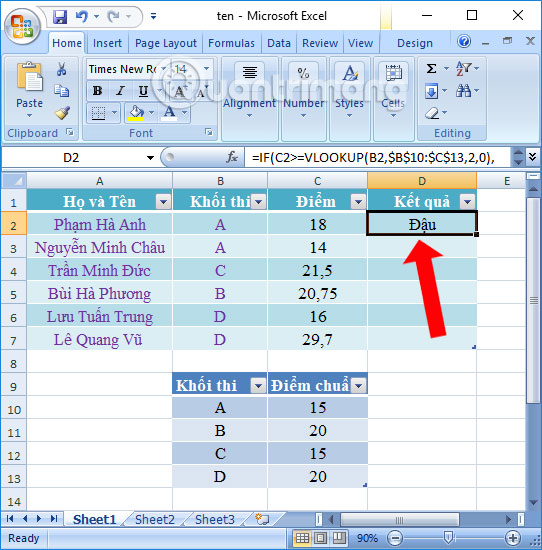
In the first result box, enter the formula to nest 2 functions: = IF (C2> = Vlookup (B2, $ B $ 10: $ C $ 13,2,0), "Beans", "Slide" .

In which C2> = Vlookup with C2 is the Score column that the students have achieved. When C2> = Vlookup satisfies the condition, it will produce a Bean result, otherwise it will not be satisfied.

Next to B2, $ B $ 10: $ C $ 13.2,0 is the group column reference located in column B and the second and line order is 10 to the expenditure column in column C with the final value in line 13.

2, 0 with 2 is the value of column 2 from the reference column in the reference table. 0 is if the value of Vlookup function cannot be found, then returns 0.

Note, to display the listed characters $ you need to localize as usual then press F4.

How to combine Vlookup function with If function in Excel Picture 2

Step 2:

When you press Enter we will get the result for the first student, Bean, which corresponds to the benchmark below. The first student gets 18 points higher with the A-grade benchmark, so the result will be the Beans as shown.

How to combine Vlookup function with If function in Excel Picture 3

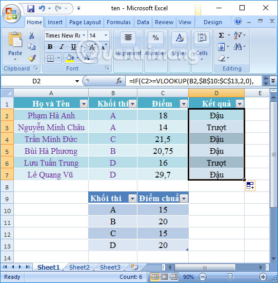
To perform the results for the remaining students, simply drag the results in the first cell down the lines of the Results column. Finally we will be evaluated as shown in the figure.

How to combine Vlookup function with If function in Excel Picture 4

Combining two Vlookup functions and such If function will save you time in finding conditional values, without having to filter the value in turn according to the VLOOKUP function and then proceed to the If function. The search table must have at least 2 columns, 1 column contains search criteria, 1 column is the value of that condition.

See more:

1. How to use the SUMIF function in Excel
2. These are the most basic functions in Excel that you need to understand
3. How to print Excel on an A4 page

I wish you all success!