The following article gives you detailed instructions on how to show / hide chart labels in Excel 2013.

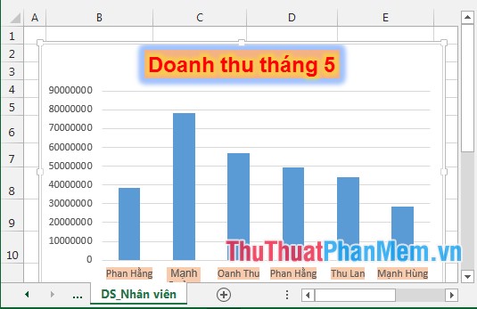
For example, the following chart has been created:

1. Want to add detailed sales for employees displayed right on the chart do the following:
- Click on the chart -> Design -> Add Chart Element -> Data labels -> select the data placement, for example, choose OutSide End :
- Revenue data results show after the end of the data column:
2. Show more Legend tags.
2.1 Display of the Legend label.
- Click on the chart -> Design -> Add Chart Element -> Legend -> choose a label location, for example choose Top:
- The label results showing the chart content are displayed:
2.2 Edit the labels.
To edit the label -> click on the label name, for example, here edit the revenue label .
Step 1: Click on the label to edit -> Format -> Shape Styles -> select the features to adjust the frame of the label:
+ Shape Fill: Fill the background for the label frame.
+ Shape OutLine: Paint the border for the frame of the label.
+ Shape Effects: Create effects for frames of labels.
Step 2: Edit the text content in the label:
Click on the label to edit -> Format -> WordArt Styles -> select the following format styles:
+ Text Fill: Coloring text.
+ Text Outline: Coloring borders for text.
+ Text Effects: Create effects for text.
- In addition to the above, double-click the label name -> Format Legend dialog box displayed -> customize the properties for the label in this dialog box:
Step 3: Change the font, font size for labels. If you think the label is a bit small or want to change the font, do the following:
- Right-click on the label -> Select Font:
- The Font dialog box appears -> change the options for labels in the dialog box -> finally click OK to finish.
- After performing the above steps, the results are:
- If you do not want to display the Legend, click on the chart -> Design -> Add Chart Element -> Legend -> None the label is automatically removed on the chart:
The above is a detailed guide on how to hide / show chart labels in Excel 2013.
Good luck!
