Hide and show gridlines in Excel

The following article guides you in detail how to show gridlines in charts in Excel 2013.

Example of creating a gridless chart:

Hide and show gridlines in Excel Picture 2

To display gridlines in the chart do the following:

1. Display grid lines in the chart:

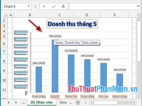
Step 1: Click on the chart -> Design -> Add Chart Element -> GridLine -> click Primary Major Horizontal to display the horizontal grid lines:

Hide and show gridlines in Excel Picture 3

After choosing the result:

Hide and show gridlines in Excel Picture 4

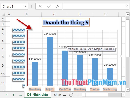
Step 2: Click the chart -> Design -> Add Chart Element -> GridLine -> click Primary Major Vertical to display vertical grid lines:

Hide and show gridlines in Excel Picture 5

If you want smaller grid lines, do the following:

+ Click on the chart -> Design -> Add Chart Element -> GridLine -> click Primary Minor Horizontal to display horizontal grid lines with small size:

Hide and show gridlines in Excel Picture 6

+ Similar to the grid lines have small vertical dimensions. After choosing the result:

Hide and show gridlines in Excel Picture 7

2. Edit the grid lines of the chart:

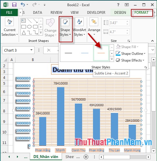
- Click on the grid of the chart -> Format -> Shape Styles -> choose the colors and effects for the grid of the chart in the section:

+ Shape Outline: Create color borders for the grid.

+ Shape Effects: Create effects for the grid.

- After modifying the grid lines the results are:

Hide and show gridlines in Excel Picture 8

3. Hide the grid lines of the chart.

- Click on the chart -> Design -> Add Chart Element -> GridLine -> click again on the selected objects to display on the chart (as shown below, all Gridline objects are not displayed) :

Hide and show gridlines in Excel Picture 9

The above is a detailed guide on how to show grid lines in a chart in Excel 2013.

Good luck!