Steps to use Pareto chart in Excel

Pareto chart in Excel will display in descending form in each column of data and automatically arrange the data displayed in the table. The following article will guide you how to use Pareto chart in Excel.

Instructions for using Pareto charts in Excel

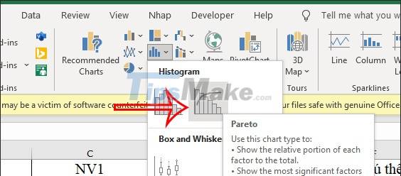
Step 1:

First you enter the data into the Excel table, then black out the entire data table. Continue to click on the Insert item and then look down at the Chart section, click on the chart icon and then select the Pareto chart in Excel.

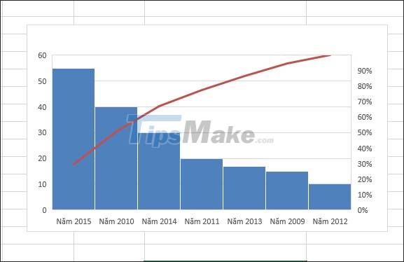
Step 2:

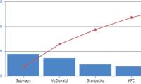
Soon you will see the Pareto chart created as shown below.

Step 3:

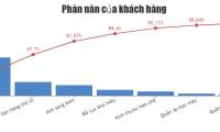
Next we enter a name for the chart in the Chart Title box. Then click the plus icon at the chart to display the selection interface of the elements appearing in the chart.

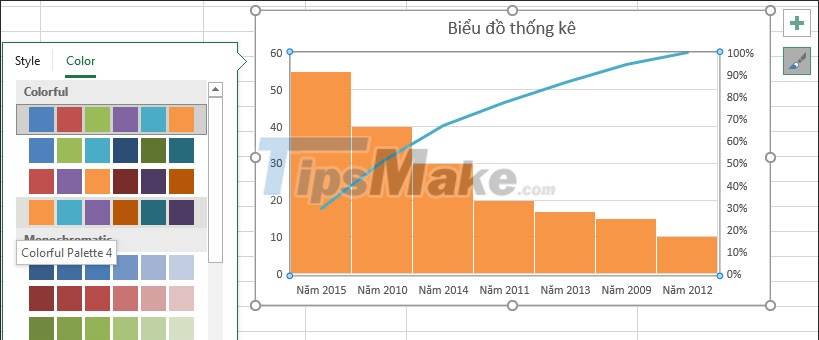
Step 4:

To adjust the display interface for the Pareto chart in Excel, click on the brush icon. This will display the interface with 2 items, Style and Color.

You can rely on this table to quickly adjust the appearance of the chart.

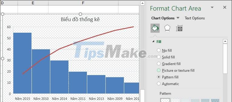
Step 5:

If you want to expand more customization for the chart, double click on the white area in the chart frame. Then on the right edge of the screen will display the interface as shown below.

Then we will have many options to change the chart such as choosing a background image for the chart, for example.

Kareem Winters

Update 23 September 2021