The SUM function is too basic, use SUMIFS instead!

You've been using the SUM function for years. It adds numbers, it does its job, and you probably don't think much about it. But while you're fiddling with filters and building messy support columns, Excel is waiting for you.

 

There's a smarter function, hiding right in plain sight, that can do the heavy lifting for you.

Why is using the SUM function alone not enough?

SUM in spreadsheets is the equivalent of an open invitation: It includes everything in the total, regardless of whether it belongs there or not. This is perfect when you just need to quickly sum columns, but in real-world work, you rarely need to add everything up.

Imagine you're a school administrator staring at a giant Excel spreadsheet filled with thousands of student records. You want to know the total score for a student, say John, on each test. With the SUM function alone, that would mean you'd have to manually find every row that John appears in, add up his scores one by one, and hope you didn't miss a single cell.

=SUM(C2,C4,C6,.)

This formula is tedious, error-prone, and gets worse as your dataset gets larger.

SUM doesn't distinguish between a column name, department, or product line. It simply adds up whatever numbers you pass in. This is fine for simple lists, but when you want to differentiate John's results from Sarah's results, or filter out all but one department, SUM falls short.

SUMIFS , on the other hand, is designed for this purpose. Instead of adding up all the data in sight, it asks you which numbers belong to the sum. The SUMIFS formula looks like this:

 

=SUMIFS(C2:C10,A2:A10,"John")

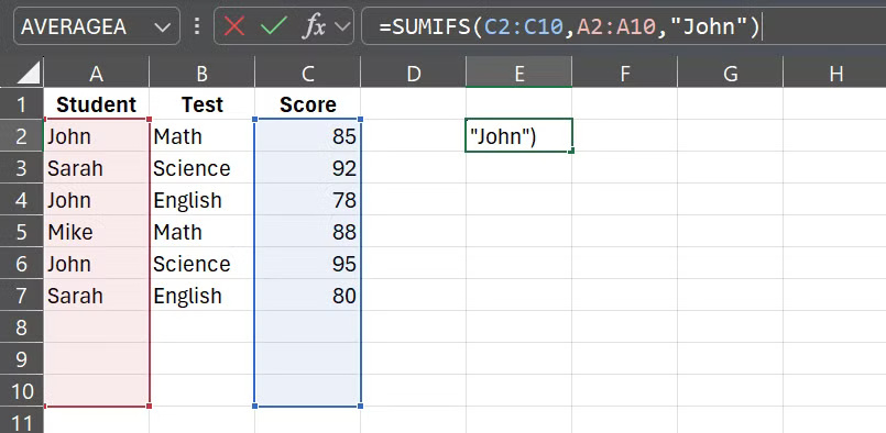
In simple terms, this formula tells Excel to look at the names in column A, find all the rows that contain the word "John," and then add up the matching scores from column C. There's no filtering, manual scanning, or support columns required—just one formula.

And it's not just for student data. Imagine tracking project costs by department, analyzing sales by region, or calculating commissions by salesperson and region. SUM will force you to work around the complexity, but SUMIFS will give you totals based on conditions you specify.

Now think about when your criteria change, which they always do. Maybe you don't want this quarter's totals anymore; you want last month's totals. Maybe you want to exclude a certain product line, or only include orders over a certain value. With SUM, you'd have to filter and select the ranges again. With SUMIFS, you just change the criteria and the formula adjusts automatically.

Smarter SUMIFS for real-world work

The syntax of the SUMIFS function is designed to handle multiple conditions at once and sum only the values ​​that meet all of them:

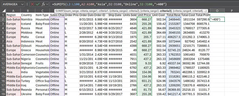
=SUMIFS (sum_range, criteria_range1, criteria1, criteria_range 2, criteria2, [criteria_range3, criteria3], …)

At first glance, it might seem a bit complicated. But when you break it down, it's actually very simple: You tell Excel to add the numbers in the specified sum_range , but only if criteria1 is true in criteria_range1 , and criteria2 is true in criteria_range2 , and so on.

 

Note : There is also SUMIF, which works the same way but only allows a single condition. People often use SUMIFS, even with one condition, because if they need to add another condition later, they don't need to rewrite the formula.

Here is a real-world example of the SUMIFS function with sales data:

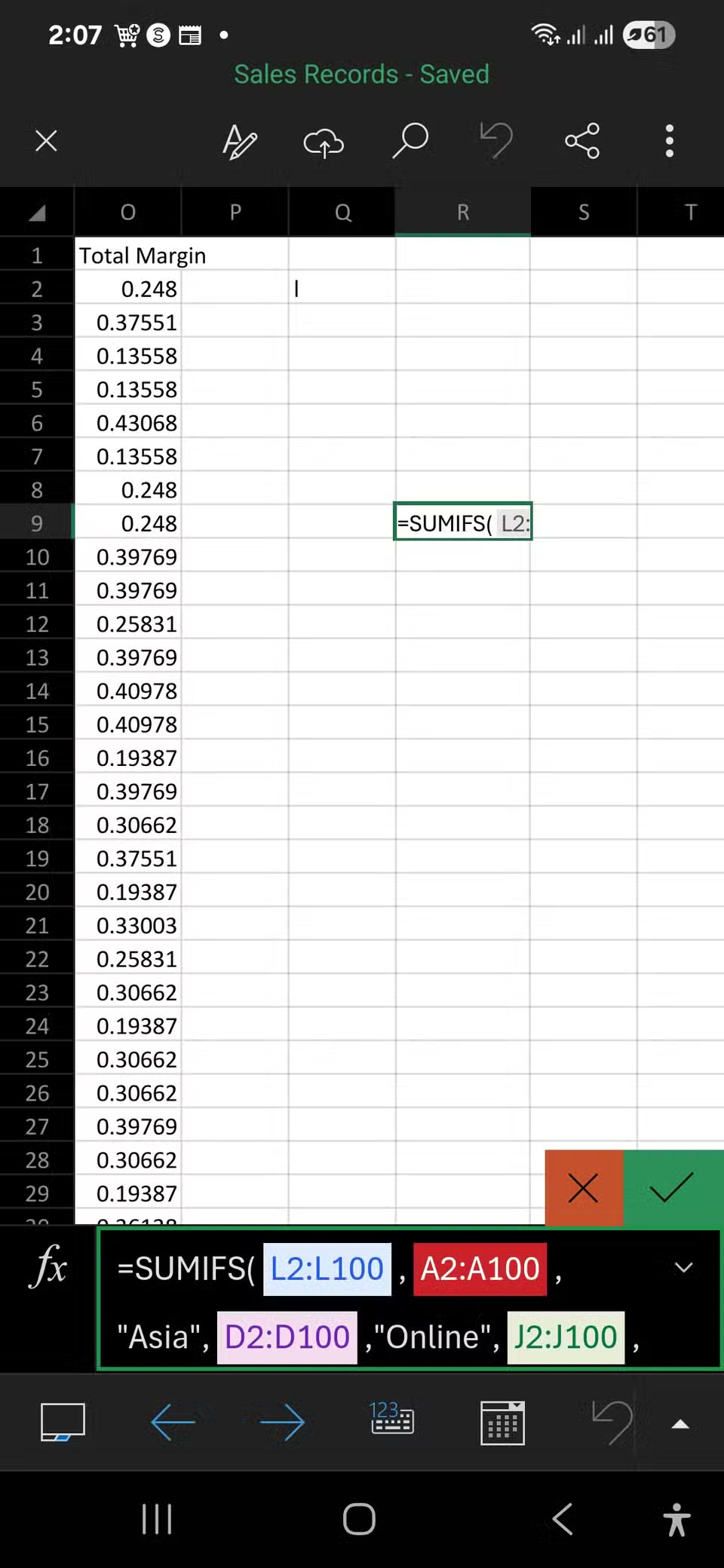
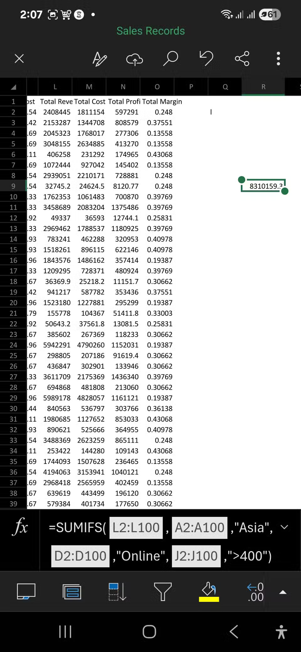
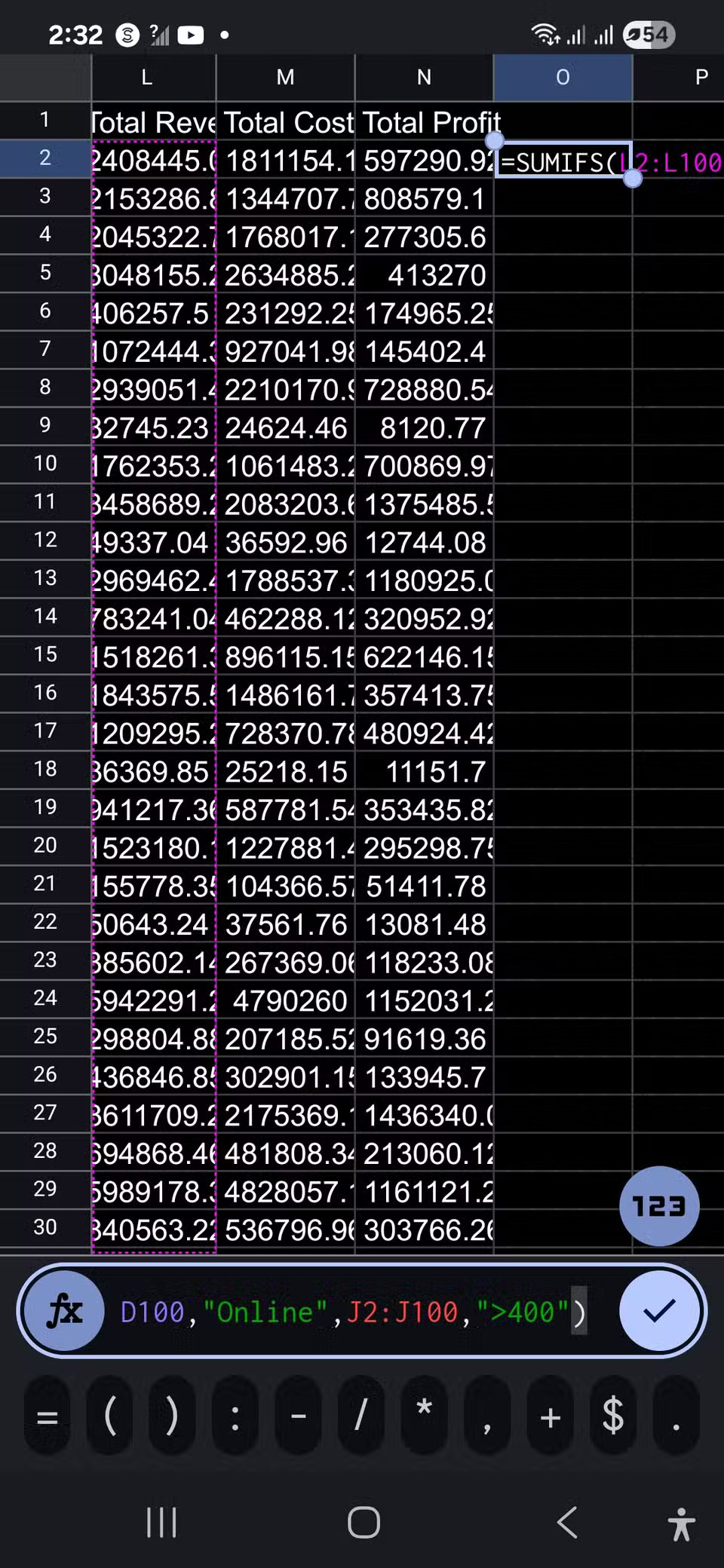
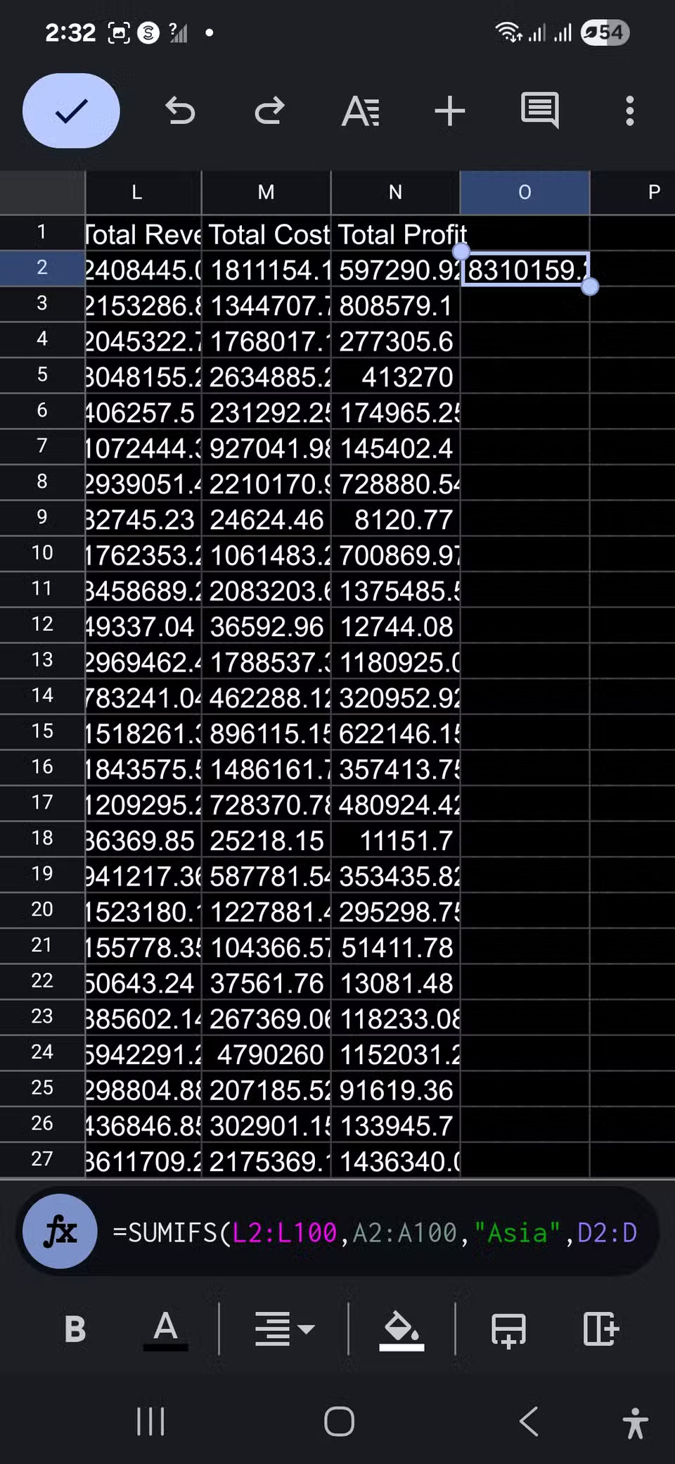
=SUMIFS (Revenue, Region, "East", Sales Channel, "Online", Price, ">500") =SUMIFS(L2:L100,A2:A100,"Asia",D2:D100,"Online",J2:J100,">400")

Basically, this formula tells Excel to go through the revenue column (in L2:L100) and add the values, but only if the region (in A2:A100) is Asia, the sales channel (in D2:D100) is online, and the price (in J2:J100) is greater than $500.

You can continue adding more criteria—country, date, salesperson, order priority, product line—and Excel will check each one. Only rows that meet all the criteria are included in the total. SUMIFS can handle up to 127 criteria, which is more than enough for even the most complex reports.

The best part is that the formula isn't static. If your data changes, like a row meets a condition, the formula will automatically update. This is great for tracking sales by region, summarizing costs by category, or tracking inventory by product type.

And if you're wondering, dates aren't a problem for SUMIFS. You can use it to sum after (or before) a specific number of days with a simple formula, like this:

=SUMIFS (Revenue, Order Date, ">=1/1/2016") =SUMIFS(N2:N100,F2:F100,">=1/1/2016")

The only detail to note is that when your criteria is not a number - such as a date or text - you need to enclose it in quotes.

SUMIFS works in all modern versions of Excel, going back to Excel 2007, and works just fine whether you're using the desktop app, Excel Online, or even the mobile app. The formula is also fully supported in Google Sheets, if you prefer that over Excel, both on the web and in the mobile app.

No matter where you work, SUMIFS is a reliable upgrade over the traditional SUM formula.