
The following article provides detailed instructions for you to aggregate data in groups in Excel.

With a large amount of data, statistical data is very complicated. Here, Excel 2013 supports the Subtotal feature, which helps you to aggregate data by group, thereby producing a more detailed, complete and accurate report:
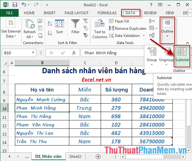
Step 1: Click the mouse at any cell in the data range you want to aggregate -> Data -> Outline -> Subtotal:
Step 2: The Subtotal dialog box appears as follows:
- Item Add each change in: Select the field to be grouped, for example, here select the group by domain.
- Use Function: Select the function to use for summarizing, for example, use the function to calculate the average value Average -> calculate the average value of the number and revenue of employees.
- Add subtotal to section: Select the data field to sum, here calculate the average value of the number and revenue to be checked in columns D and E:
Step 3: After clicking OK, the result is as shown in the picture:
- You can customize the data more visually:
- The data is aggregated by region, ending 3 regions as the aggregate value for the North, Central and South.
- Excel supports Subtotal 's minimized toolbar in the upper left corner of the screen. With a large volume of data, click No. 1 -> Show the average of the total data of all groups:
- Click the number 2 -> to display aggregated values for each group and the combined total value for all groups:
The above is a detailed guide on how to aggregate data in groups in Excel 2013.
Good luck!