How to Unhide Rows in Excel

Method 1 of 3:

Unhiding All Hidden Rows

Open the Excel document. Double-click the Excel document that you want to use to open it in Excel.
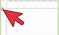
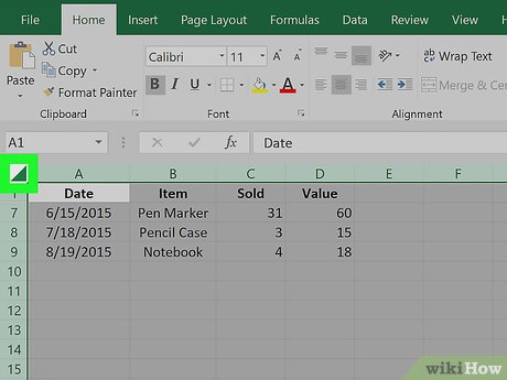Click the "Select All" button. This triangular button is in the upper-left corner of the spreadsheet, just above the 1 row and just left of the A column heading. Doing so selects your entire Excel document.
1. You can also click any cell in the document and then press Ctrl+A (Windows) or ⌘ Command+A (Mac) to select the whole document.
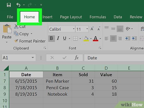Click the Home tab. This tab is just below the green ribbon at the top of the Excel window.
1. If you're already on the Home tab, skip this step.
Click Format. This option is in the "Cells" section of the toolbar near the top-right of the Excel window. A drop-down menu will appear.
Select Hide & Unhide. You'll find this option in the Format drop-down menu. Selecting it prompts a pop-out menu to appear.
Click Unhide Rows. It's in the pop-out menu. Doing so immediately causes any hidden rows to appear in the spreadsheet.
1. You can save your changes by pressing Ctrl+S (Windows) or ⌘ Command+S (Mac).

Method 2 of 3:

Unhiding a Specific Row

Open the Excel document. Double-click the Excel document that you want to use to open it in Excel.
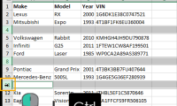
Find the hidden row. Look at the row numbers on the left side of the document as you scroll down; if you see a skip in numbers (e.g., row 23 is directly above row 25), the row in between the numbers is hidden (in 23 and 25 example, row 24 would be hidden). You should also see a double line between the two row numbers.^[1]
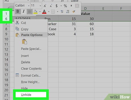
Right-click the space between the two row numbers. Doing so prompts a drop-down menu to appear.
1. For example, if row 24 is hidden, you would right-click the space between 23 and 25.
2. On a Mac, you can hold down Control while clicking this space to prompt the drop-down menu.
Click Unhide. It's in the drop-down menu. Doing so will prompt the hidden row to appear.
1. You can save your changes by pressing Ctrl+S (Windows) or ⌘ Command+S (Mac).
Unhide a range of rows. If you notice that several rows are missing, you can unhide all of the rows by doing the following:
1. Hold down Ctrl (Windows) or ⌘ Command (Mac) while clicking the row number above the hidden rows and the row number below the hidden rows.
2. Right-click one of the selected row numbers.
3. Click Unhide in the drop-down menu.

Method 3 of 3:

Adjusting Row Height

Understand when this method is necessary. One form of hiding rows involves the height of the row(s) in question to be so short that the row effectively disappears. You can reset the height of all spreadsheet rows to "14.4" (the default height) to address this.
Open the Excel document. Double-click the Excel document that you want to use to open it in Excel.
Click the "Select All" button. This triangular button is in the upper-left corner of the spreadsheet, just above the 1 row and just left of the A column heading. Doing so selects your entire Excel document.
1. You can also click any cell in the document and then press Ctrl+A (Windows) or ⌘ Command+A (Mac) to select the whole document.
Click the Home tab. This tab is just below the green ribbon at the top of the Excel window.
1. If you're already on the Home tab, skip this step.
Click Format. This option is in the "Cells" section of the toolbar near the top-right of the Excel window. A drop-down menu will appear.
Click Row Height…. It's in the drop-down menu. This will open a pop-up window with a blank text field in it.
Enter the default row height. Type 14.4 into the pop-up window's text field.
Click OK. Doing so will apply your changes to all rows in the spreadsheet, thus unhiding any rows which were "hidden" via their height properties.
1. You can save your changes by pressing Ctrl+S (Windows) or ⌘ Command+S (Mac).

Jessica Tanner

Update 05 March 2020

You should read it

May be interested

How to Change from Lowercase to Uppercase in Excel
microsoft's excel spreadsheet program has several functions to make your text type-case consistent. if you have a series of names that is in the lowercase, you can use 'flash fill' function to capitalize names in excel 2013. if you need...
How to Create a Custom Macro Button in Excel
macros in excel can save a great deal of time with repetitive tasks. by assigning macros to custom buttons, you can save even more time by bringing your macro only one-click from execution. click tools → customize.
How to Freeze Cells in Excel
this wikihow teaches you how to freeze specific rows and columns in your microsoft excel worksheet. freezing rows or columns ensures that certain cells remain visible as you scroll through the data. if you want to easily edit two parts of...
How to Round in Excel
this wikihow teaches you how to round the value of a cell using the round formula, and how to use cell formatting to display cell values as rounded numbers. enter the data into your spreadsheet.
How to Create a Timeline in Excel
excel isn't heavy on the graphics, but there are still several ways to create a timeline. if you have excel 2013 or later, you can even create it automatically from a pivot table. earlier versions will have to rely on smartart, templates,...
How to Create Pivot Tables in Excel
pivot tables are interactive tables that allow the user to group and summarize large amounts of data in a concise, tabular format for easier reporting and analysis. they can sort, count, and total the data, and are available in a variety...

How to Unhide Rows in Excel

Unhiding All Hidden Rows

Unhiding a Specific Row

Adjusting Row Height

You should read it

May be interested

Office information