How to Create Pivot Tables in Excel

Part 1 of 3:

Building the Pivot Table

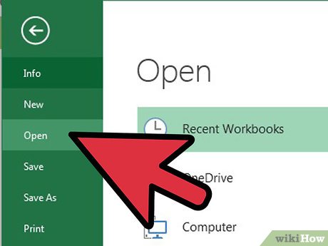Load the spreadsheet you want to create the Pivot Table from. A Pivot Table allows you to create visual reports of the data from a spreadsheet. You can perform calculations without having to input any formulas or copy any cells. You will need a spreadsheet with several entries in order to create a Pivot Table.
1. You can also create a Pivot Table in Excel using an outside data source, such as Access. You can insert the Pivot Table in a new Excel spreadsheet.
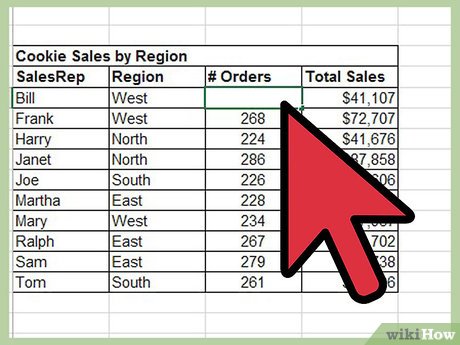
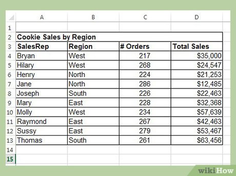Ensure that your data meets the needs of a pivot table. A pivot table is not always the answer you are looking for. In order to take advantage of the pivot table features, your spreadsheet should meet some basic criteria:^[1]
1. Your spreadsheet should include at least one column with duplicate values. This basically just means that at least one column should have repeating data. In the example discussed in the next section, the "Product Type" column has two entries: "Table" or "Chair".
2. It should include numerical information. This is what will be compared and totaled in the table. In the example in the next section, the "Sales" column has numerical data.
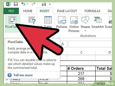Start the Pivot Table wizard. Click the "Insert" tab at the top of the Excel window. Click the "PivotTable" button on the left side of the Insert ribbon.
1. If you are using Excel 2003 or earlier, click the Data menu and select PivotTable and PivotChart Report...
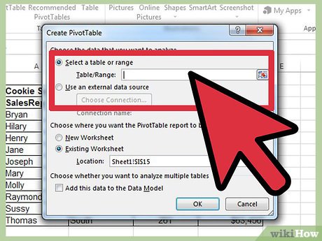Select the data you want to use. By default, Excel will select all of the data on your active spreadsheet. You can click and drag to choose a specific part of the spreadsheet, or you can type the cell range in manually.
1. If you are using an external source for your data, click the "Use an external data source" option and click Choose Connection.... Browse for the database connection saved on your computer.
Select the location for your Pivot Table. After selecting your range, choose your location option from the same window. By default, Excel will place the table on a new worksheet, allowing you to switch back and forth by clicking the tabs at the bottom of the window. You can also choose to place the Pivot Table on the same sheet as the data, which allows you to pick the cell you want it to be placed.^[2]
1. When you are satisfied with your choices, click OK. Your Pivot Table will be placed and the interface will change.

Part 2 of 3:

Configuring the Pivot Table

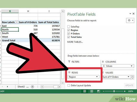Add a row field. When creating a Pivot Table, you are essentially sorting your data by rows and columns. What you add where determines the structure of the table. Drag a field from the Field List on the right onto the Row Fields section of the Pivot Table to insert the information.
1. For example, your company sells two products: tables and chairs. You have a spreadsheet with the number (Sales) of each product (Product Type) sold in your five stores (Store). You want to see how much of each product is sold in each store.
2. Drag the Store field from the field list into the Row Fields section of the Pivot Table. Your list of stores will appear, each as its own row.
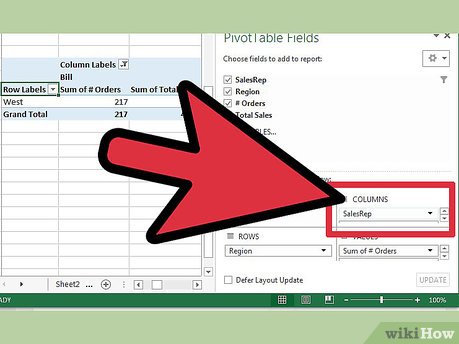Add a column field. Like the rows, the columns allow you to sort and display your data. In the above example, the Store field was added to the Row Fields section. To see how much of each type of product was sold, drag the Product Type field to the Column Fields section.
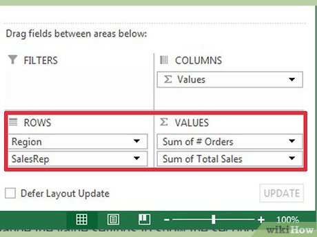
Add a value field. Now that you have the organization laid out, you can add the data to be displayed in the table. Click and drag the Sales field into Value Fields section of the Pivot Table. You will see your table display the sales information for both of your products in each of your stores, with a Total column on the right.^[3]
1. For all of the above steps, you can drag the fields into the corresponding boxes below the Fields list on the right side of the window instead of dragging them onto the table.
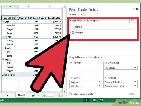
Add multiple fields to a section. Pivot tables allow you to add multiple fields to each section, allowing for more minute control over how the data is displayed. Using the above example, say you make several types of tables and several types of chairs. Your spreadsheet is records whether the item is a table or chair (Product Type), but also the exact model of the table or chair sold (Model).
1. Drag the Model field onto the Column Fields section. The columns will now display the breakdown of sales per model and overall type. You can change the order that these labels are displayed by clicking the arrow button next to the field in the boxes in the lower-right corner of the window. Select "Move Up" or "Move Down" to change the order.
Change the way data is displayed. You can change the way values are displayed by clicking the arrow icon next to a value in the Values box. Select "Value Field Settings" to change the way the values are calculated. For example, you could display the value in terms of a percentage instead of a total, or average the values instead of summing them.
1. You can add the same field to the Value box multiple times to take advantage of this. In the above example, the sales total for each store is displayed. By adding the Sales field again, you can change the value settings to show the second Sales as percentage of total sales.
Learn some of the ways that values can be manipulated. When changing the ways values are calculated, you have several options to choose from depending on your needs.
1. Sum - This is the default for value fields. Excel will total all of the values in the selected field.
2. Count - This will count the number of cells that contain data in the selected field.
3. Average - This will take the average of all of the values in the selected field.
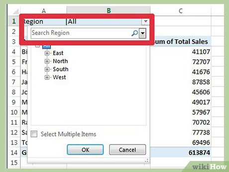Add a filter. The "Report filter" area contains the fields that enable you to page through the data summaries shown in the pivot table by filtering out sets of data. They act as the filters for the report. For example, setting your Store field as the filter instead of a Row Label will allow you to select each store to see individual sales totals, or see multiple stores at the same time.

Part 3 of 3:

Using the Pivot Table

Sort and filter your results. One of the key features of the Pivot Table is the ability to sort results and see dynamic reports. Each label can be sorted and filtered by clicking the down arrow button next to the label header. You can then sort the list or filter it to only show specific entries.^[4]
Update your spreadsheet. Your pivot table will automatically update as you modify the base spreadsheet. This can be great for monitoring your spreadsheets and tracking changes. .
Change your pivot table around. Pivot tables make it extremely easy to change the location and order of fields. Try dragging different fields to different locations to come up with a pivot table that meets your exact needs.
1. This is where the pivot table gets its name. Moving the data to different locations is known as "pivoting" as you are changing the direction that the data is displayed.
Create a Pivot Chart. You can use a Pivot Chart to show dynamic visual reports. Your Pivot Chart can be created directly from your completed Pivot Table, making the chart creation process a snap.^[5]

Marvin Fry

Update 05 March 2020

You should read it

May be interested

12 steps to pivot startup
if many pivot startup startups, there may be more startups. pivot is a secret to survive. learning how to pivot will help you save your startup from failure and keep growing for a long time.
How to Create a Timeline in Excel
excel isn't heavy on the graphics, but there are still several ways to create a timeline. if you have excel 2013 or later, you can even create it automatically from a pivot table. earlier versions will have to rely on smartart, templates,...
How to Merge in Excel
microsoft office excel offers a variety of features for customizing tables and charts that contain important information. the program also provides efficient ways to combine and summarize data from multiple files and worksheets. common methods for merging in excel include merging by location, by category, using formulas, or the program's pivot table feature. learn how to consolidate in excel so that your information shows up in the master sheet and can be referenced whenever you need to report.
Instructions to delete 0, hide 0 in Excel
when working on excel, with statistics tables with 0, users can completely hide or hide the number 0 with the tools available on the system.
How to draw charts in Excel
drawing diagrams on excel are basic and often done, when displaying data based on tables or comparing figures together.
How to create tables and tables in Word - Instructions on how to create tables and tables in Word 2007, 2010, 2013, 2016
how to create tables and tables in word - instructions on how to create tables and tables in word 2007, 2010, 2013, 2016. tables help your data presented scientifically easier to see and understand than using text simple version to show off. in this article help the b
PIVOT clause in SQL Server
in sql server (transact-sql), the pivot clause allows cross tabulation to pass data from one table to another.
How to update Excel PivotTable data
in the process of using pivot table, updating data is a necessary operation so that the data in the pivot table is also updated.
MS Excel - Lesson 4: Working with lines, columns, sheets
in addition to the content of tables in excel, operations with lines, columns and sheets in this program are also important. in this article, tipsmake.com will guide you to simple operation to add or remove lines, columns or sheets in excel tables.
Table in CSS
tables in html can become much more beautiful thanks to css.

How to Create Pivot Tables in Excel

Building the Pivot Table

Configuring the Pivot Table

Using the Pivot Table

You should read it

May be interested

Office information