How to Change from Lowercase to Uppercase in Excel
Microsoft's Excel spreadsheet program has several functions to make your text type-case consistent. If you have a series of names that is in the lowercase, you can use 'flash fill' function to capitalize names in Excel 2013. If you need...
Method 1 of 4:
Using the Uppercase Function
-
 Type in a series of names or text in a column in your worksheet. Your text can be in any case when using this function. It will change the text in the cell to all uppercase letters.
 -
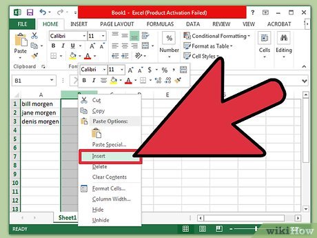
 Add a column to the right of your text column. Click on the letter on the top of the text column. Right click and select 'Insert.'
 -
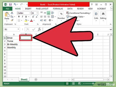
 Move your cursor into the cell to the right of the first data you want to capitalize. You will place a formula with the uppercase function in this cell.
 -
 Press the function button in the top toolbar. It is a blue epsilon symbol and looks like the letter 'E.' The formula bar (fx) will be highlighted so that you can type in your function.
 -
 Select the text function labeled 'UPPER' or type in the word 'UPPER' next to the equals sign in your formula bar.
- When you press the function button, the word 'SUM' may automatically appear. If this happens, replace 'SUM' with 'UPPER' to change the function.[1]
-
 Type the cell location in parenthesis next to the word UPPER. If you were using the first column and row for your data, your function bar would read '=UPPER(A1).'
 -
 Press 'Enter.' The text in cell A1 should appear in cell B1 in all-uppercase letters.
 -
 Click your cursor on the little box in the bottom right corner of the cell. Drag the box to the bottom of the column. This will fill in the series so that each cell in the first column is copied to the second column in the uppercase.
 -
 Check that all of the text has been correctly copied into the second column. Highlight the column above the correct text by clicking on the letter above the column. Click on the 'Edit' menu and click 'Copy,' and then click the 'Edit' drop down menu and select 'Paste Values.'
- This process will allow you to replace the formula with the value, so that you can delete the first column of text.
-
 Check that the same text reappears in the column. Delete the first column by right clicking the letter above the column. Select 'Delete' from the drop down list.
Method 2 of 4:
Using the Proper Name Function
-
 Enter your text into the first column of your spreadsheet. This function will help you to capitalize the first letter of your text in each cell.
 -
 Add a new column. Right click on the letter heading the first column. Select 'Insert' in the drop down menu.
 -
 Move your cursor to the cell to the right of the first text entry. Click the formula button. This is the blue epsilon symbol in the top horizontal toolbar.
 -
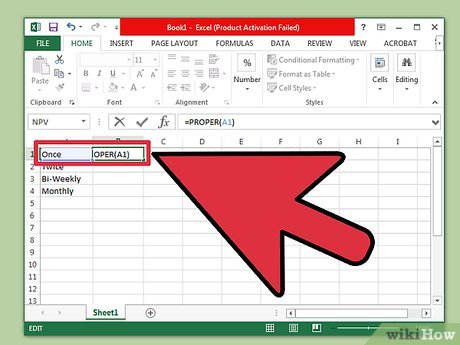
 Click on the formula bar. It is a query bar next to the 'fx' sign just above your spreadsheet. Type the word 'PROPER' after the equals sign.
- If the word 'SUM' automatically appeared in the formula bar, replace it with the word 'PROPER' to change the function.
-
 Type the first cell location of your text in parenthesis next to the word 'PROPER.' For example, it should read '=PROPER(A1).'
 -
 Press 'Enter.' The first letter of each word in the cell should be capitalized in the column to the right of the original text. The rest of the text will be lowercase.[2]
 -
 Grab the box in the lower right corner of the cell. Drag it down the column until you are at the bottom of your original text column. Release the mouse, and all the text should have copied with the first letters capitalized.
 -
 Click on the letter at the top of your replacement column to select the entire column. Click the 'Edit' menu and select 'Copy.' Then, click the drop down menu on the Paste button and select 'Paste Values.'
- The formula based cells will be replaced with the text, so that you can delete the first column.
-
 Right click on the first column. Select 'Delete' to get rid of it and leave the replacement values with proper cases.
Method 3 of 4:
Using Flash Fill in Excel 2013
-
 Use this section if your series is a list of proper names. It will need to be written in Excel in the lowercase to use this method. The flash fill function can read and change names so that the first letter of the first and last name is capitalized.
 -
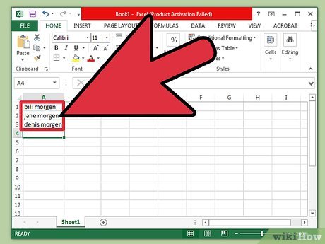
 Complete your list of names using lowercase letters. Enter them in a single column. Leave a blank column to the right of the list of names.
- If you don't currently have a blank column to the right of your list of names, right click on the lettered column above your list of names. Select 'Insert' and a new empty column will appear to the right.
-
 Click on the cell to the right of the first name that is listed. For example, if your first lowercase name were in cell A1, you would go to cell B1.
 -
 Type the same name as the cell in A1, but include proper capitalization of first and last names. For example, if the first cell says 'joe biggins,' type 'Joe Biggins' in the cell to the right. Press 'Enter.'
 -
 Go to the 'Data' menu and select 'Flash Fill.' It will learn the pattern and make a similar change in the data series. You can also use the short cut code, 'Control' and the letter 'E' to activate Flash Fill.[3]
 -
 Delete the column with the lowercase names. To avoid duplication, click on the top of the original lowercase column. Right click and press 'delete' to get rid of it and leave the list with proper cases.
- Make sure Flash Fill has worked on your whole list before deleting.
Method 4 of 4:
Using Word
-
 An alternative to writing Excel formulas to change the case which is very quick is this:
 -
 Open a blank Word document
 -
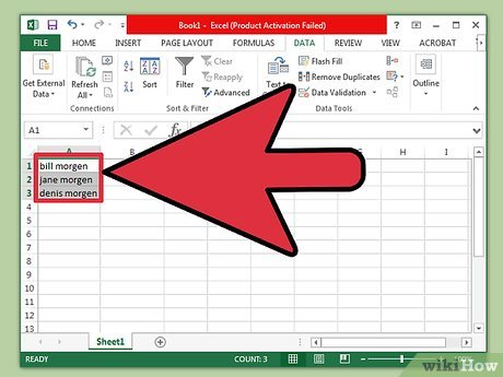
 In Excel, highlight the cells that you want to change the case in
 -
 Copy the cells (Control "C")
 -
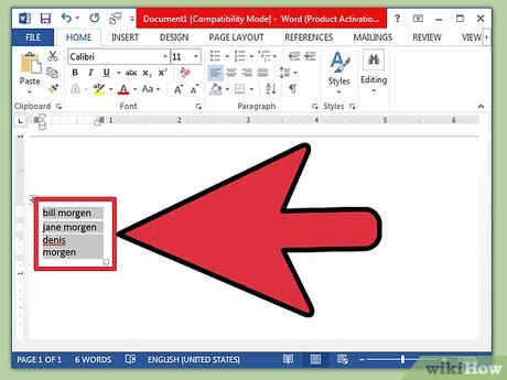
 Paste it into the Word document (Control "V")
 -
 Highlight all the text in the Word Document
 -
 Click on the "Change Case" dropdown menu in the "Home" tab
 -
 Choose the option you would like - Sentence case, lowercase, UPPERCASE, Capitalize Each Word, tOGGLE cASE
 -
 After the case has changed, highlight all the text and paste it back into Excel
 -
 The whole process takes a few seconds
Similar Post
- 2 Ways to convert lowercase to uppercase in Excel
- How to convert uppercase to lowercase in Excel simple and fast
- Convert lowercase to uppercase in Word, Excel
- How to convert lowercase letters to uppercase and vice versa on Word
- How to convert uppercase letters to lowercase letters in PowerPoint
- How to create drop down lists in Excel











 Instructions for using the IF function in Excel
  Adjust the spacing between columns in Word
  How to change the position of columns in Excel
  How to arrange alphabetical order in Google Sheets
  The way to sum the same codes in Excel
  How to Remove Spaces Between Characters and Numbers in Excel