How to temporarily hide rows and columns in Excel 2013

Instructions on how to temporarily hide and make appear again in one or more rows / columns in the Microsoft Excel 2013 spreadsheet.

Excel 2013 has a feature that allows temporary users to hide one or more rows / columns in an Excel spreadsheet. This feature is very useful in case you only want to print a part of the spreadsheet but do not want to delete other excess rows and columns.

Note: Cells in hidden rows and columns are still included in the table calculations.

Hide one or more rows

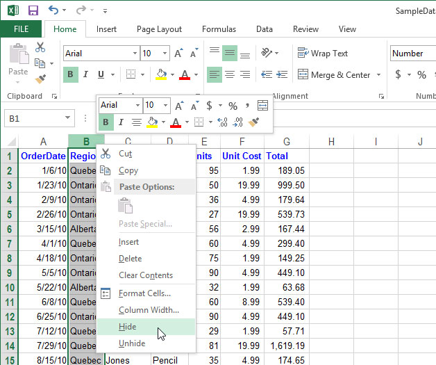
Select the rows you want to hide.

How to temporarily hide rows and columns in Excel 2013 Picture 1

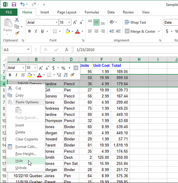
Right-click on one of the selected row titles, select 'Hide' from the menu (menu) that appears.

How to temporarily hide rows and columns in Excel 2013 Picture 2

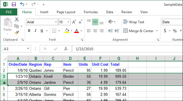
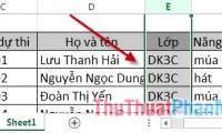
The selected rows will be pressed, including the row title.

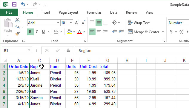
Note that rows 3 and 4 in the picture below are hidden. Separating between rows 2 and 5 (where hidden rows are located) is a bold line. When you perform other operations on the spreadsheet, this bold line will disappear. However, you can identify locations of hidden rows by viewing which row titles are missing.

How to temporarily hide rows and columns in Excel 2013 Picture 3

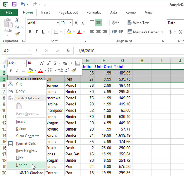
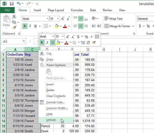
To reappear a row, you must select the row above and the row below the hidden rows. In this case, row 2 and row 5. Then right-click on the title of the selected row, press 'Unhide' from the menu that appears.

How to temporarily hide rows and columns in Excel 2013 Picture 4

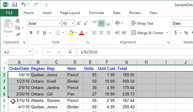
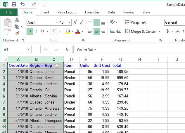
Hidden rows will reappear and be marked with the surrounding rows.

How to temporarily hide rows and columns in Excel 2013 Picture 5

Hide one or more columns

You can also easily hide one or more columns. Select the columns you want to hide, right-click one of the column headers, select 'Hide' from the menu that appears.

How to temporarily hide rows and columns in Excel 2013 Picture 6

The selected columns will disappear with the column header. The position of the pressed column is marked with a bold line.

How to temporarily hide rows and columns in Excel 2013 Picture 7

To reappear hidden columns, like with hidden rows, select the columns on the left and right of the hidden columns, right-click one of the column headers, select 'Unhide' from the menu appear.

How to temporarily hide rows and columns in Excel 2013 Picture 8

Hidden columns will reappear and be marked with the columns on the left and right of it.

How to temporarily hide rows and columns in Excel 2013 Picture 9