Instructions for coloring alternating rows and columns in Excel

Instructions on how to color alternate rows and columns in Excel using Conditional Formatting. You can do it easily on Excel versions 2007, 2010, 2013, 2016.
 

Table of Contents:
1. Done in Excel 2016
2. Done in Excel 2013 spreadsheet

1. How to alternate colors in Excel 2016

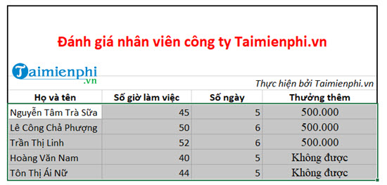
Step 1: Highlight the cells that need to be colored alternately.

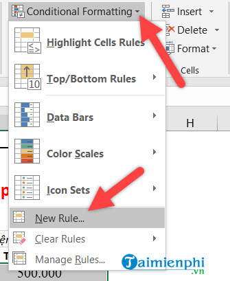
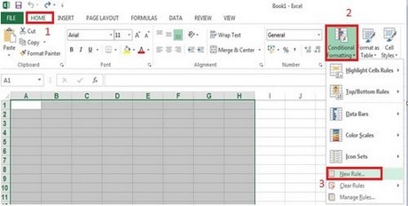
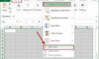
Step 2: Next, we need to do is on the Home interface of Excel, select Conditional Formatting > select New Rule.

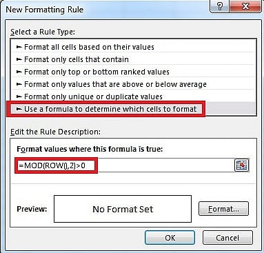
Step 3: Next, select the last line Use a formula to determine which cells to format , below we fill in =MOD(ROW(),2)>0 then click Format .

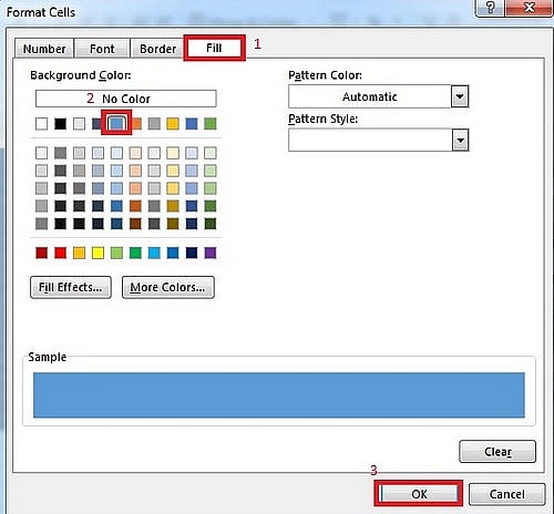
Step 4: Next, select Fill and choose the color you want.

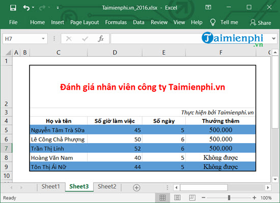
Then you just need to click OK and the result will appear as below.

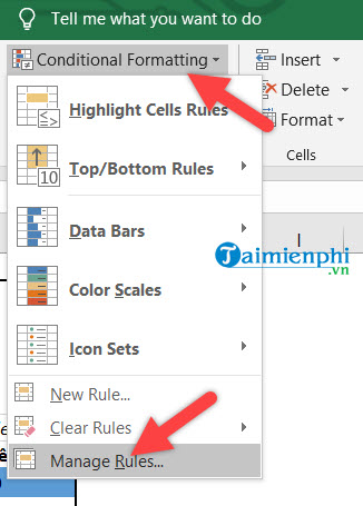
Step 5: Click Manage Rules .

Step 6: Here you will see the list of Rules just created and we just need to click to change the color.

Step 7: Continue to apply steps 3 and 4 to change the color and choose the color you want.

2. How to alternate colors in Excel 2013 spreadsheet

Step 1: Open the Excel spreadsheet that you want to color alternately.
Step 2: Color the rows on the spreadsheet with Conditional Formatting

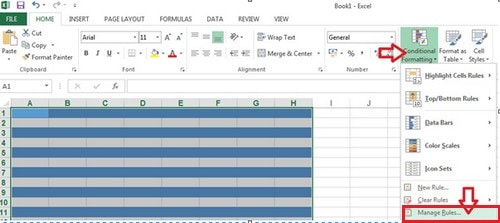
On the program interface, go to the  Home tab  of the Ribbon bar, select  Conditional Formatting in the Style group , then select  New Rule in the drop-down menu.

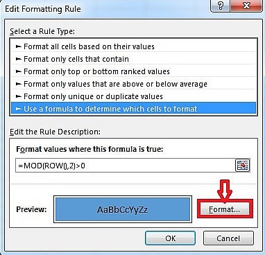
The New Formatting Rule dialog box appears. In the Format values ​​where this formula is true box , type the following formula: =MOD(ROW(),2)>0

Next, to choose the fill color for the alternating rows, click the  Format button, the Format Cells dialog box   appears, click the  Fill tab  and choose the color you want to fill (here I choose light blue). Finally, press O K to finish.

Step 3: Change the fill color on alternating lines

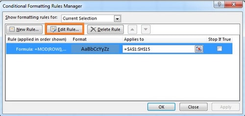
If you want to choose a different color (other than the blue above) click Conditional Formatting then click Manage Rule .

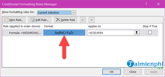
The Conditional Formatting Rule Manager dialog box  appears, select Edit Rule .

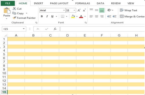
Click on the  Format box and select the color you want to change (here taimienphi chooses yellow). Then click OK to finish.

The results have changed:

Alternating colors in Excel spreadsheets not only makes it easier to distinguish data, but also makes your charts more intuitive and easier to follow. This is especially useful when you work with spreadsheets containing many rows and columns of data, helping to reduce confusion and increase work efficiency.

If you want to optimize your Excel spreadsheets further, you can try other tricks such as counting the number of words in cells, rows or columns to work with data more flexibly. Refer to tutorial articles such as how to use the LEN function in combination with the SUBSTITUTE and TRIM functions to  count the number of words in Excel  easily, helping to optimize your spreadsheets.

Samuel Daniel

Update 18 February 2025