Instructions on how to cross cells in Excel

To cross cells in Excel, you just need to use the cell adjustment tool in Excel with very simple usage features. Cross lines in Excel are very familiar, especially when you create a table in Excel to divide the title cell into 2 different contents in the same cell.

The diagonal line in an Excel cell will divide an empty cell in Excel into two parts to represent the two functions of rows and columns, and describe the two contents of columns and rows. The article below will guide you through cross-hatching cells in Excel with different versions.

Instructions for crossing cells in Excel 2016, 2019

How to cross out Excel cells from Font on the Ribbon

Step 1:

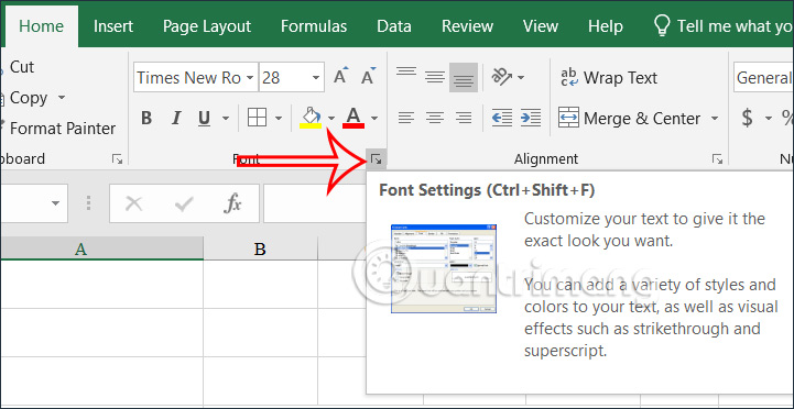
First, click on the cell that needs to divide the diagonal line in the data table. Next, the user clicks on the Home tab on the toolbar. You look down at the Font group and then click on the arrow icon as shown below.

Step 2:

Switch to the new interface, click on Border .

The user will now see the interface to draw borders for cells in Excel. You will draw a slash to the right or left depending on the content in the writing box.

You choose the direction of the crossed out box you want to use and then click OK below to create.

As a result, we have crossed cells in Excel as shown below.

How to cross out Excel cells from the right-click menu

Step 1:

Also in the cell you want to cross, right-click and select Format Cells in the displayed list.

Step 2:

This time also displays the Format Cells dialog box, click Border to choose to create borders for cells in Excel.

Step 3:

We can also choose the direction of the slashes in the cell to use for our Excel table.

How to write text in crossed out cells in Excel

Step 1:

In the slashed box you want to insert content, first double-click twice in the box with the slashed line . Next we enter the first content we want to add to the cell and then use the Space key to align to the right side of the cell.

Step 2:

Press the key combination Alt + Enter to break the line and then enter the second content for the column row in the table.

Step 3:

As a result, we will get the content in the diagonal box as shown below.

If the text in the cell is shifted up or down, you will use the alignment icon as shown below.

Instructions for removing slashes in Excel

If you do not want to use slashes in the cell, just select the delete function.

Click on the box with the crossed out box, click on the Home tab, then look down at the Editing group and click on the Clear icon . Next select Clear Format in the displayed list.

Video instructions for crossing cells in Excel 2016, 2019

How to create diagonal lines in Excel 2007

Step 1:

First of all, we have the data table below as an example. Here, I will perform the operation of dividing the first cell in the table into 2 small cells with a clear diagonal division including Area and Category. The Zone column will include all locations below. The Category column includes Product Type and Quantity.

In the cell that needs to be divided, the user right-clicks and selects Format Cells. to set up all the properties that affect this cell in the data table.

Step 2:

The Format Cells dialog box interface appears. Here, we click on the Border tab . Because the requirement here is to divide 1 Excel cell into 2 diagonal triangles, creating an Excel diagonal, we follow the steps below:

1. 1: Border tab to create a border for the table.
2. 2: Create Excel diagonal lines in two different directions, left and right. When pressing once to create a diagonal line, pressing twice to cancel that diagonal line.
3. 3: Select the diagonal style for the cell including dark and light styles or select cut lines.
4. 4: Choose to add an internal or external threading frame.
5. 5: Choose the color for the border.

Finally click OK to save the changes.

Immediately after that, you will have a table with cells with lines.

Step 3:

Finally, we just need to enter text for each created cell . Press the Space key to align the text, depending on the length and length of the text in each cell. Press the key combination Alt + Enter to enter a new line in that cell.

The final result will be a data table with the first cell forming 2 small triangles with diagonal lines as shown.

Creating 1 cell into 2 triangle cells in Excel with diagonal lines will help the table be clearer, more flexible as well as accurate in presenting content and data. Depending on the content of each table, users can customize the text content accordingly.

Jessica Tanner

Update 26 July 2024