8 ways to number Excel numbers, number Excel numbers with text

Numbering in Excel is no longer a complicated operation but one of the most basic operations when working with Excel. However, numbering in Excel does not have to be done manually, but you will have a way to automatically number in Excel, saving more time and also showing professionalism when working. Below are some ways to number sequentially in Excel for you to choose the appropriate method.

1. Numbering in Excel with the mouse

This is a very simple way to help you type numbers automatically in Excel with just one mouse click, and you can type as many numbers as you want.

First, you will number the first 2 cells , then circle those first 2 cells and see the plus symbol in the bottom right corner of the highlighted area.

8 ways to number Excel numbers, number Excel numbers with text Picture 1

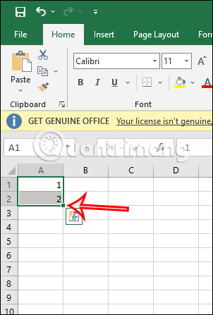
Then you just need to scroll down to the number you want to use and you're done.

8 ways to number Excel numbers, number Excel numbers with text Picture 2

In case you are numbering with odd even number , do the same. Enter the number for the first 2 boxes according to the rule you want to play, then highlight those 2 boxes and drag them down. The result of the automatically entered serial number still follows the order principle in the first 2 cells.

8 ways to number Excel numbers, number Excel numbers with text Picture 3

2. How to number Excel numbers using formulas

We will use the formula =First cell position + n according to the numbering rule you want. If numbering is consecutive, n=1 will be set.

For example, according to the image below, there will be the formula =C1+3 to automatically number in Excel according to the formula with n=3. Press Enter and the second cell is 4.

8 ways to number Excel numbers, number Excel numbers with text Picture 4

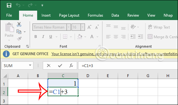
Now you will drag from the 2nd cell down to the remaining cells to number them according to the rules you have set up.

8 ways to number Excel numbers, number Excel numbers with text Picture 5

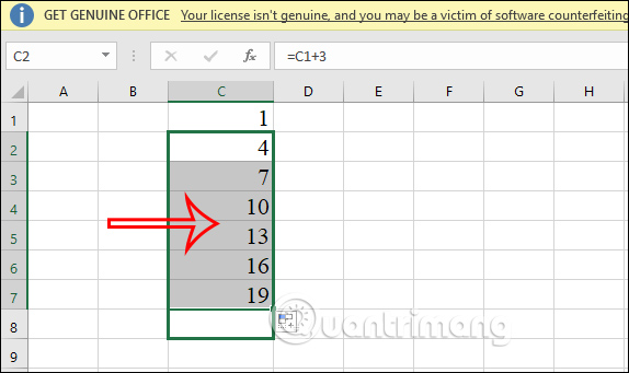
3. Use the SEQUENCE function to number in Excel

When you use the SEQUENCE function in Excel to number sequentially, it is very simple and not complicated. Note, the SEQUENCE Excel function only applies to Office 365 and Excel online versions.

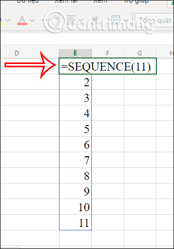
You just need to follow the formula =SEQUENCE(Number of rows to be numbered) and press Enter.

8 ways to number Excel numbers, number Excel numbers with text Picture 6

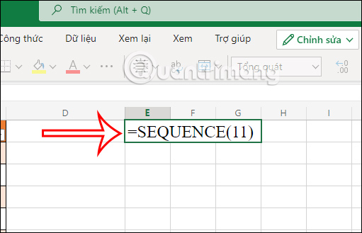
Immediately the row is returned with the value you entered for the SEQUENCE function in Excel.

8 ways to number Excel numbers, number Excel numbers with text Picture 7

4. How to use the ROW function for sequential numbering in Excel

To use the ROW function for numbering in Excel, you will need to follow the ROW() formula . For example, in the image below, you will start entering number 1 from row number 5, then you will need to enter the formula =ROW() - 4. The result of cell number 1 will be displayed.

8 ways to number Excel numbers, number Excel numbers with text Picture 8

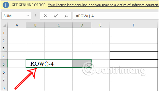
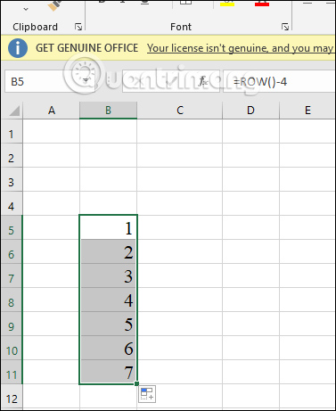
Now you just need to scroll down from number 1 below to enter the next number.

When using the ROW numbering function, if rows are added or deleted, the numbering will be automatically adjusted.

8 ways to number Excel numbers, number Excel numbers with text Picture 9

5. How to number Excel sequentially except for blank rows

There will be cases where you need to number the Excel data table, when there are blank rows if we do not delete Excel blank lines. Then you will have to implement the SUBTOTAL function nested with the IF function.

We will do this with the data table below when we need sequential numbering, but minus the blank lines.

8 ways to number Excel numbers, number Excel numbers with text Picture 10

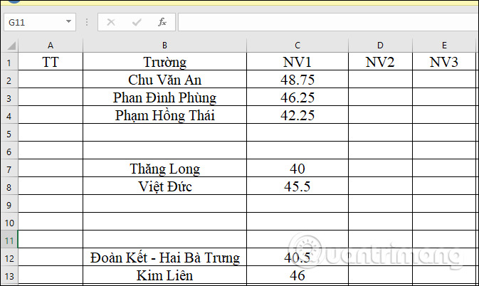
We have the box function syntax = IF(logical_test; [value_if_true]; [value_if_false]; SUBTOTAL(function_num; ref1;.) . In which:

1. logical_test: Condition of IF function.
2. [value_if_true]: Return value if condition is true.
3. [value_if_false]: Return value if condition is false.
4. function_num: The function is understood as a numeric value (Enter 3 is equivalent to the COUNTA function).
5. ref1;.: Area containing sequence numbers.

Applying to the table, we will have the formula =IF(B2="","",SUBTOTAL(3,$B$2:B2)) . Where SUBTOTAL(3,$B$2:B2)) means:

1. 3 is function_num which is the COUNTA function in SUBTOTAL that counts the number of non-empty cells.
2. $B$2:B2 is a numbered area, you must use the $ value to lock the first cell.

IF(B2="","",SUBTOTAL(3,$B$2:B2)) means:

1. B2="","" If cell B2 is empty, it will not be numbered.
2. SUBTOTAL(3,$B$2:B2)) If cell B2 has a value, the SUBTOTAL function will be used.

Now in the first cell A2 , enter the formula =IF(B2="","",SUBTOTAL(3,$B$2:B2)) and press Enter.

8 ways to number Excel numbers, number Excel numbers with text Picture 11

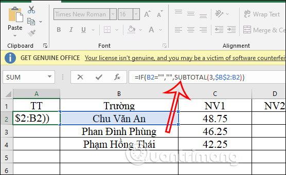
Immediately after that, the number 1 will be displayed. You will continue to drag to the remaining cells to number them automatically in Excel.

As a result, we will see that the Excel numbers are ignored and empty Excel lines do not display numbers, and the cells with data are given the next number.

8 ways to number Excel numbers, number Excel numbers with text Picture 12

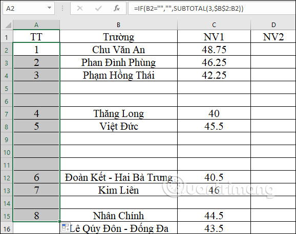
So you have many ways to number in Excel. Depending on how the data table you work with, we choose the appropriate numbering style.

6. Numbering in Excel using Fill

Step 1:

First, you enter all the data into the table, leaving the columns that need to be numbered sequentially. In the example table below, there will be sequential numbers in the STT column. Next, enter the first cell as 1 in the STT column, then highlight the area that needs to be numbered starting from 1 as shown below.

8 ways to number Excel numbers, number Excel numbers with text Picture 13

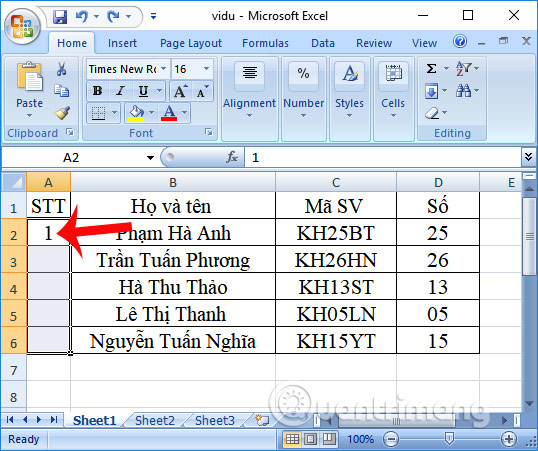
Step 2:

Look up the Ribbon and find the Home tab . Then look at the Editing section, select Fill , then select Series.

8 ways to number Excel numbers, number Excel numbers with text Picture 14

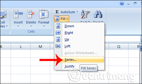
Step 3:

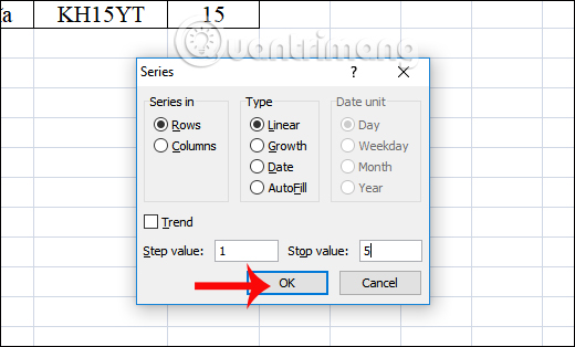
In the Series dialog box that appears, users take turns customizing the following items:

1. Series in: check Rows if numbered in rows, or Columns if numbered in columns.
2. Type: Here there will be a number of options for sequential numbering including Linear to number sequentially in ascending style, Growth sequential numbering to be progressive, Date serial number to date, AutoFill to automatically fill in sequential numbers. .
3. Step value: choose the distance between 2 ordinal numbers in the column.
4. Stop value: number the line to which position.

According to the requirements of the article, in the Print Series section, I will select Columns to number the columns in order, in the Type section, select Linear as an ascending number, the Step value here will be entered as 1 and the Stop value at the final position is 5. . Click OK to save the settings.

8 ways to number Excel numbers, number Excel numbers with text Picture 15

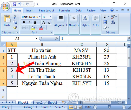
Finally you get the result that the cells are numbered automatically.

8 ways to number Excel numbers, number Excel numbers with text Picture 16

7. Numbering in Excel using Fill Series

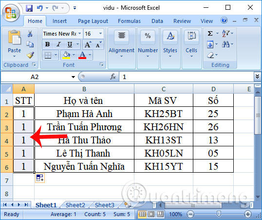
Another way also uses the Fill Series feature in Excel , but should be applied in case you do not need to customize the numbering as much as the method above. This method requires dragging the sequential number column. In the STT column, enter the first cell as 1 and then drag down the remaining cells. Thus, the remaining order cells will all be 1.

8 ways to number Excel numbers, number Excel numbers with text Picture 17

Click on the plus icon as shown below to open the Auto Fills Options section , then select Fill Series . The sequence number will immediately be automatically filled in to the last sequence number position.

8 ways to number Excel numbers, number Excel numbers with text Picture 18

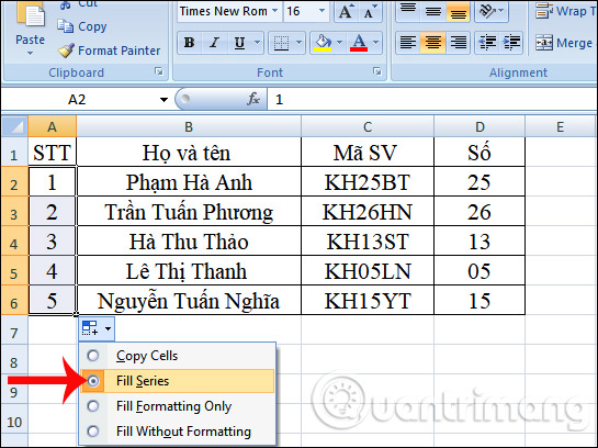
Instead of dragging the mouse to the position where the serial number is needed, through the Fill Series feature, the serial number will be entered automatically. Besides, users also have an additional custom number when numbering in columns such as sequential numbering, numbering for columns or rows,.

8. How to number Excel numbers with letters

In addition to the usual Excel letter numbering, many data also require you to number with letters. For example, you will see Excel numbering with letters like A1, A2, A3, etc. If used according to normal operations, it will not display the order with letters you want, but must have a few more. Other operations.

Method 1: Number Excel numbers with letters via Format Cells

Step 1:

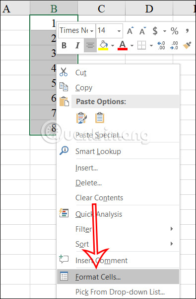
First, users number the data cells as usual using the above methods. Next, highlight the entire number cell and then right-click and select Format Cells in the displayed list.

8 ways to number Excel numbers, number Excel numbers with text Picture 19

Step 2:

Displaying a new dialog box, the user clicks on the Custom tab , then types "A"# in the Type box and clicks OK to finish. If you add more letters to the numbered box, enter them in quotation marks.

8 ways to number Excel numbers, number Excel numbers with text Picture 20

Step 3:

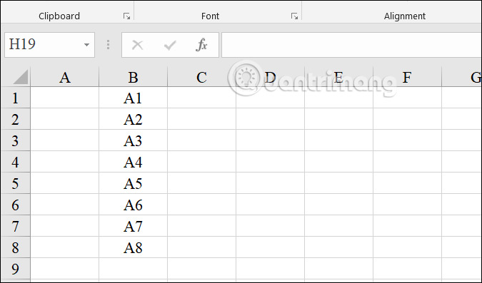
As a result, we will get a series of numbered cells with text as shown below.

8 ways to number Excel numbers, number Excel numbers with text Picture 21

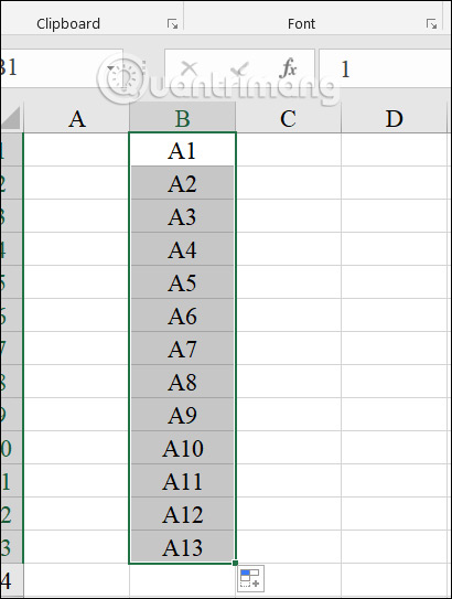
You continue to scroll down to continue typing the serial number box with other letters for the data.

8 ways to number Excel numbers, number Excel numbers with text Picture 22

Method 2: Use the sequential numbering formula with Excel letters

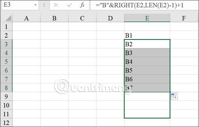
First, you will manually type the order box with the letter B1 in cell E2 as shown below. Note that you cannot type the order in the first cell in each column. Then enter the formula ="B"&RIGHT(E2,LEN(E2)-1)+1 . In there:

1. Function RIGHT(text,[num_chars]).
2. Text: The text string containing the characters you want to extract.
3. Num_chars: Specify the number of characters you want the RIGHT function to extract.
4. LEN function (text)
5. Text: is the data cell you want to count

Then press Enter to display the results.

8 ways to number Excel numbers, number Excel numbers with text Picture 23

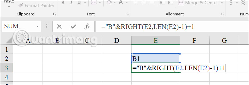
Then you will also get the next numbered box. We just need to drag from this cell down to the remaining cells to get a sequential numbering sequence with letters as shown below.

8 ways to number Excel numbers, number Excel numbers with text Picture 24

David Pac

Update 24 July 2024