How to format data based on other cell conditions in Excel

However, there are also cases where you will format the condition based on the data of another cell. Basically, the conditional formatting operation based on another cell is the same as when you create conditional formatting. Below are detailed instructions for other cell-based conditional formatting on Zalo.

Guide to Conditional Formatting Based on Other Columns Excel

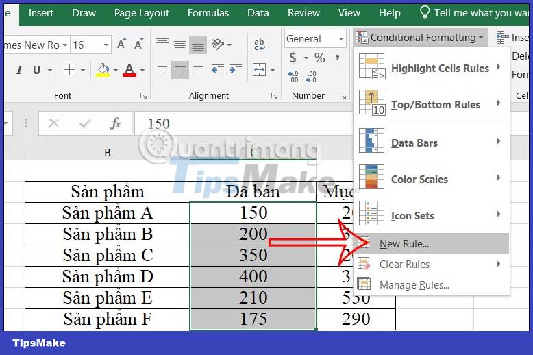
Step 1:

First we create a data table on Excel as usual. Now you highlight the data column you want to create conditional formatting based on another column. Then click on Conditional Formatting and select New Rule .

Step 2:

Now display the interface to set the format. At the list of format types, scroll down and click Use a formula to determine which cells to format .

Next at Format values ​​where this formula is true , enter the format condition as =C33 >= $D33 . Where C33 is the starting cell of the column to be formatted, D33 is the column of conditional data provided that column C33 is greater than or equal to the data in column D33.

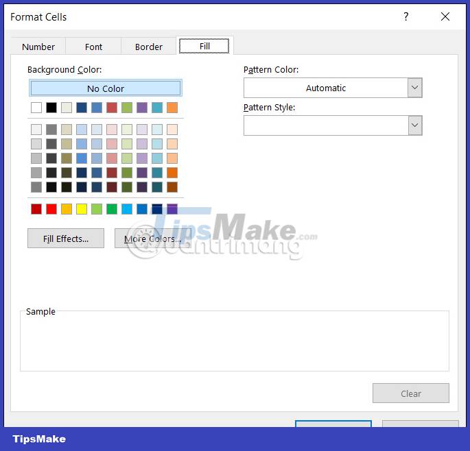
Step 3:

You click on the Format button and then click on the Fill tab to choose the color you want to set for the data formatted according to the condition. After setting up, click the OK button to save the format for the data according to the conditions you choose.

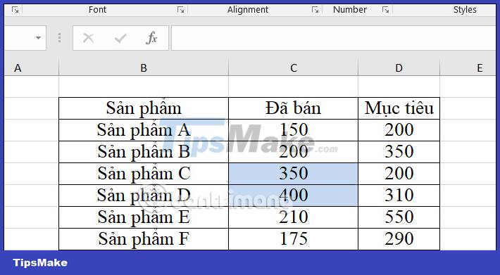
Step 4:

As a result, you will see the data cells are formatted based on the conditions you set. Cells with higher values ​​are marked for easy identification.

How to format Excel data based on another cell

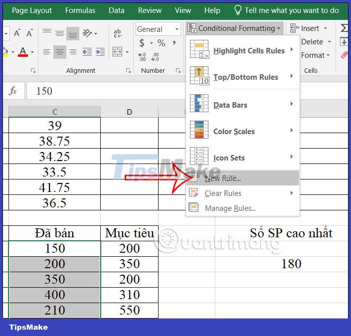
Step 1:

First you also create the data table and the value cell you want to use as a condition. Next, highlight the column you want to format the data, then click on Conditional Formatting and select New Rule .

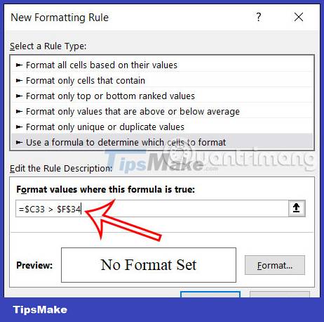
Switch to the new interface, click Use a formula to determine which cells to format .

Next, enter the condition =$C33 > $F$34 with cell F34 as the conditional data for you to format for column C33.

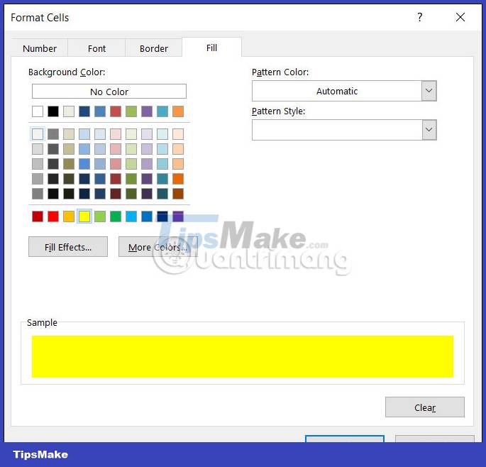
Step 2:

Click the Format button and then click the Fill tab to choose a color for the data. Finally, click OK to proceed with formatting the data according to the value condition in the selected cell.

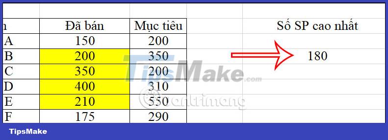
As a result, we will see data cells that are greater than or equal to the condition value cell you have selected.

Isabella Humphrey

Update 04 August 2023