How to color formula cells in Excel automatically
Coloring formula cells in Excel helps us quickly identify cells that use formulas in long data tables.
Table of Contents
Formulas in Excel or functions in Excel like Vlookup and SUM functions help to calculate data or process tables more easily and quickly. And of course, when processing the data table, it will need manipulations to check operations, or some cases we need to lock Excel formulas to avoid editing. However, with long data tables, finding the correct formula cell is relatively time consuming. If so, the user can color the Excel formula cell automatically, quickly identify which data areas in the table use the formula for faster processing. The following article will guide you how to color formula cells in Excel
1. How to color formula cells in Excel automatically
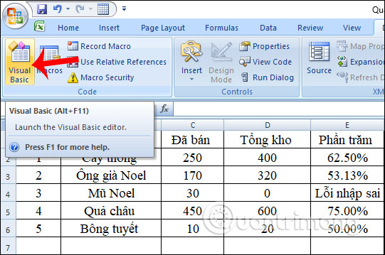
At the Excel table interface to find the formula cell, we click on the Developer tab and then select Visual Basic as shown below.
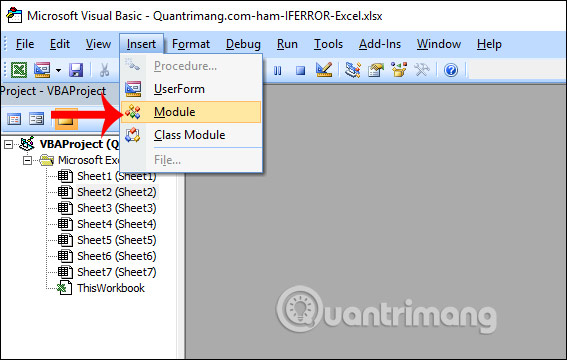
Display the VBA interface, click Insert and select Module to display the code input interface.
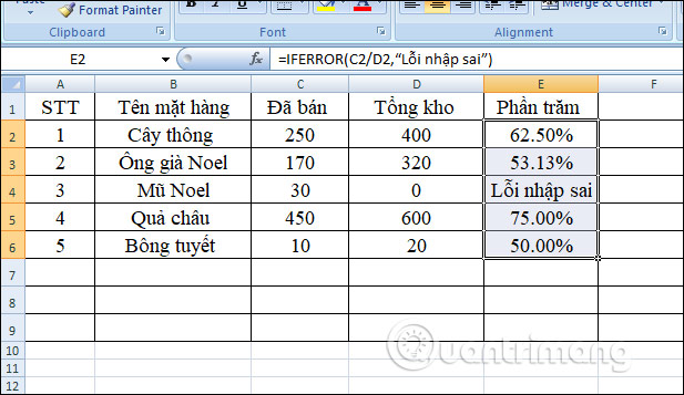
Next, you enter the code below to filter and search for cells that use formulas in the table.Notice at the line of code Rng.Interior.ColorIndex = 36 , the number 36 is the color code so we can change to another color code if we want to use another color. Click Run to run the code.
Sub SelectFormulaCells() 'Updateby20140827 Dim Rng As Range Dim WorkRng As Range On Error Resume Next xTitleId = 'KutoolsforExcel' Set WorkRng = Application.Selection Set WorkRng = Application.InputBox('Range', xTitleId, WorkRng.Address, Type:=8) Set WorkRng = WorkRng.SpecialCells(xlCellTypeFormulas, 23) Application.ScreenUpdating = False For Each Rng In WorkRng Rng.Interior.ColorIndex = 50 Next Application.ScreenUpdating = True End Sub
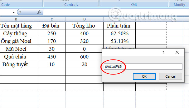
Next, you localize the data in the KutoolsforExcel dialog interface and click OK to color.
The results of the cells that use the formula are colored as shown below. The color depends on the color code the user entered in the code.

2. Localize formulas in Excel
If you do not want to color in a table, just quickly highlight the range of data using the formula, just use the Go To Special tool .
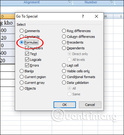
We highlight the whole table and press the F5 key to open the Go To dialog box, then click Special to expand the custom.
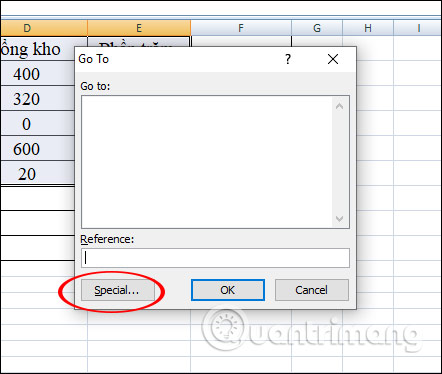
Next to display the table, tick Formulas and click OK to identify the formula.
Then the data area using the zoned formula is identified as below.
See more:
- 4 basic steps for alternating coloring of lines in Microsoft Excel
- 4 basic steps to color alternating columns in Microsoft Excel
Was this article helpful?
Your feedback helps us improve.
Related Articles
 How to calculate and color blank cells in Excel4 minutes read
 How to Add Numbers Automatically in Excel5 minutes read
 How to automatically calculate and copy formulas in Excel4 minutes read
 How to indent the line in Excel2 minutes read
 How to enter a text into multiple Excel cells at the same time3 minutes read
 Merge cells in Excel7 minutes read
Reader Comments 0
Sign in with email or Google to join the discussion.