Insert and edit charts in Excel
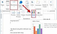
Instructions on how to insert and edit charts in Excel. To insert a chart, follow these steps: Step 1: Select the data to create a chart. The example here wants to create a sales chart of the employees. Go to the Insert tab - illustration - Chart -
The following article details you how to insert and edit charts in Excel 2013.

To insert a chart, follow these steps:
Step 1: Select the data to create a chart. The example here wants to create a sales chart of the employees. Go to the Insert tab -> illustration -> Chart -> select the type of chart you want to create:

Step 2: After selecting the chart type -> data has been shown on the chart:

Step 3: After creating the chart, you need to adjust the chart to look better and more intuitive. Click on the chart -> click on the Chart Element icon to customize the components in the chart:

- For example, when selecting the Data Labels icon -> the quantity value is displayed corresponding to the columns on the chart:

- Or when selecting a Legend chart again:

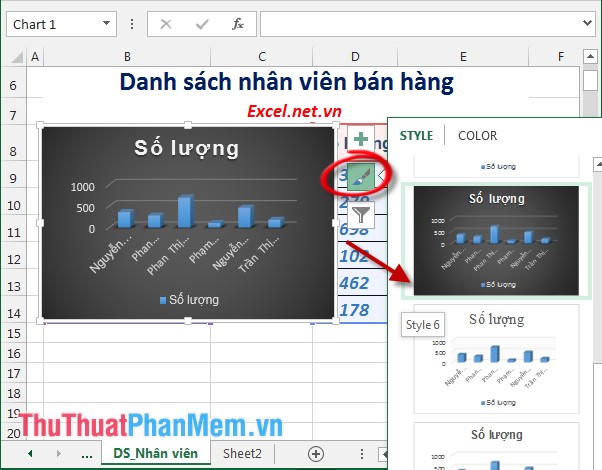
Step 4: Change the chart style -> click on the chart -> select the Chart Style icon on the chart to re-select the chart style and color for the chart:
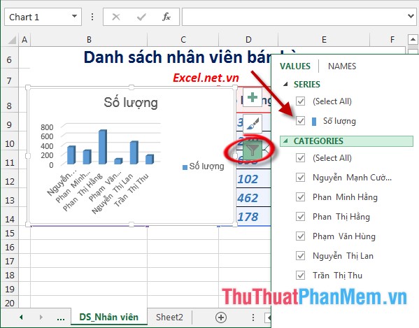
Step 5: Excel 2013 supports additional filtering features on the chart -> click on the chart -> select the Chart Filters icon -> precursor filter data by ticking on the items as shown:
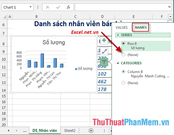
- Or you can filter data by name by selecting the Names tab .
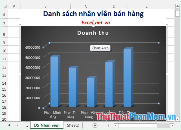
- So just a few simple operations you have created the chart:
Above is detailed instructions for inserting and editing charts in Excel 2013.
Good luck!
Was this article helpful?
Your feedback helps us improve.
Related Articles
 How to draw a map chart on Excel4 minutes read
 Insert and edit charts in Word2 minutes read
 How to fix chart position in Excel2 minutes read
 Instructions on how to create charts in Excel professional7 minutes read
 How to draw charts in Excel6 minutes read
 Insert and edit flowcharts (SmartArt) in Excel2 minutes read
Reader Comments 0
Sign in with email or Google to join the discussion.